| .github/workflows | ||
| img | ||
| src | ||
| test | ||
| .gitignore | ||
| LICENSE | ||
| package.yaml | ||
| README.md | ||
| Setup.hs | ||
| stack.yaml | ||
| WhyHaskellMatters.iml | ||
Why Haskell Matters
This is an early draft work in progress article.
Motivation
Haskell was started as an academic research language in the late 1980ies. It was never one of the most popular languages in the software industry.
So why should we concern ourselves with it?
Instead of answering this question directly I'd like to first have a closer look on the reception of Haskell in the software developers community:
A strange development over time
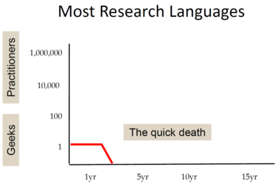
In a talk in 2017 on the Haskell journey since its beginnings in the 1980ies Simon Peyton Jones speaks about the rather unusual life story of Haskell.
First he shows a chart representing the typical life cycle of research languages. They are often created by a single researcher (who is also the single user) and most of them will be abandoned after just a few years:
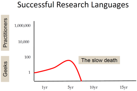
A more successful research language gains some interest in a larger community but will still not escape the ivory tower and typically will die within ten years:
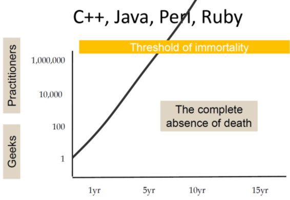
On the other hand we have popular programming languages that are quickly adopted by large numbers of users and thus reach "the threshold of immortality". That is the base of existing code will grow so large that the language will be in use for decades:
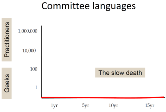
In the next chart he rather jokingly depicts the sad fate of languages designed by committees. They simply never take off:
Finally he presents a chart showing the Haskell timeline:
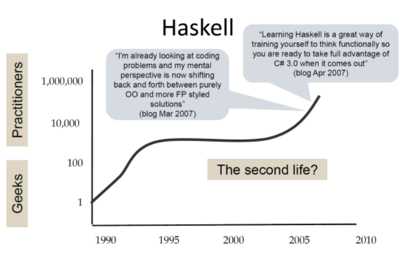
The development shown in this chart is rather unexpected and unusual: Haskell started as a research language and was even designed by a committee; so in all probability it should have been abandoned long before the millennium!
But instead it gained some momentum in the early years followed by a rather quiet phase during the decade of OO hype (Java was released in 1995). And then again we see a continuous growth of interest since about 2005. I'm writing this in early 2020 and we still see this trend.
Being used versus being discussed
Then Simon Peyton Jones points out another interesting characteristic of the reception of Haskell in recent years. In statics that rank programming languages by actual usage Haskell is typically not under the 30 most active languages. But in statistics that instead rank programming languages by the volume of discussions on the internet Haskell typically scores much better (often in the top ten).
So why does Haskell keep to be such a hot topic in the software development community?
A very short answer might be: Haskell has a number of features that are clearly different from those of most other programming languages. Many of these features have proven to be powerful tools to solve basic problems of software development elegantly.
Therefore over time other programming languages have adopted parts of these concepts (e.g. pattern matching or type classes). In discussions about such concepts the origin from Haskell is mentioned and differences between the Haskell concepts and those of other languages are discussed. Sometimes people are encouraged to have a closer look at the source of these concepts to get a deeper understanding of their original intentions. That's why we see a growing number of developers working in Python, Typescript, Scala, Rust, C++, C# or Java starting to dive into Haskell.
A further essential point is that Haskell is still an experimental laboratory for research in areas such as compiler construction, programming language design, theorem-provers, type systems etc. So inevitably Haskell will be a topic in the discussion about these approaches.
In the next section we want to study some of the most distinguishing features of Haskell.
So what exactly are those magic powers of Haskell?
Haskell doesn't solve different problems than other languages. But it solves them differently.
-- unknown
In this section we will examine the most outstanding features of the Haskell language. I'll try to keep the learning curve moderate and so I'll start with some very basic concepts.
Even though I'll try to keep the presentation self-contained it's not intended to be an introduction to the Haskell language (have a look at Learn You a Haskell if you are looking for enjoyable tutorial).
Functions are First-class
In computer science, a programming language is said to have first-class functions if it treats functions as first-class citizens. This means the language supports passing functions as arguments to other functions, returning them as the values from other functions, and assigning them to variables or storing them in data structures.[1] Some programming language theorists require support for anonymous functions (function literals) as well.[2] In languages with first-class functions, the names of functions do not have any special status; they are treated like ordinary variables with a function type.
quoted from Wikipedia
We'll go through this one by one:
functions can be assigned to variables exactly as any other other values
Let's have a look how this looks like in Haskell. First we define some simple values:
-- define constant `aNumber` with a value of 42.
aNumber :: Integer
aNumber = 42

-- define constant `aString` with a value of "hello world"
aString :: String
aString = "Hello World"
In the first line we see a type signature that defines the constant aNumber to be of type Integer.
In the second line we define the value of aNumber to be 42.
In the same way we define the constant aString to be of type String.
Next we define a function square that takes an integer argument and returns the square value of the argument:
square :: Integer -> Integer
square x = x * x
Definition of a function works exactly in the same way as the definition of any other value.
The only thing special is that we declare the type to be a function type by using the -> notation.
So :: Integer -> Integer represents a function from Integer to Integer.
In the second line we define function square to compute x * x for any Integer argument x.
Ok, seems not too difficult, so let's define another function double that doubles its input value:
double :: Integer -> Integer
double n = 2 * n
support for anonymous functions
Anonymous functions, also known as lambda expressions, can be defined in Haskell like this:
\x -> x * x
This expression denotes an anonymous function that takes a single argument x and returns the square of that argument. The backslash is read as λ (the greek letter lambda).
You can use such as expressions everywhere where you would use any other function. For example you could apply the
anonymous function \x -> x * x to a number just like the named function square:
-- use named function:
result = square 5

-- use anonymous function:
result' = (\x -> x * x) 5
We will see more useful applications of anonymous functions in the following section.
Functions can be returned as values from other functions
function composition
Do you remember function composition from your high-school math classes?
Function composition is an operation that takes two functions f and g and produces a function h such that
h(x) = g(f(x))
The resulting composite function is denoted h = g ∘ f where (g ∘ f )(x) = g(f(x)).
Intuitively, composing functions is a chaining process in which the output of function f is used as input of function g.
So looking from a programmers perspective the ∘ operator is a function that
takes two functions as arguments and returns a new composite function.
In Haskell this operator is represented as the dot operator .:
(.) :: (b -> c) -> (a -> b) -> a -> c
(.) f g x = f (g x)
The brackets around the dot are required as we want to use a non-alphabetical symbol as an identifier.
In Haskell such identifiers can be used as infix operators (as we will see below).
Otherwise (.) is defined as any other function.
Please also note how close the syntax is to the original mathematical definition.
Using this operator we can easily create a composite function that first doubles a number and then computes the square of that doubled number:
squareAfterDouble :: Integer -> Integer
squareAfterDouble = square . double
Currying and Partial Application
In this section we look at another interesting example of functions producing
other functions as return values.
We start by defining a function add that takes two Integer arguments and computes their sum:
-- function adding two numbers
add :: Integer -> Integer -> Integer
add x y = x + y
This look quite straightforward. But still there is one interesting detail to note:
the type signature of add is not something like
add :: (Integer, Integer) -> Integer
Instead it is:
add :: Integer -> Integer -> Integer
What does this signature actually mean?
It can be read as "A function taking an Integer argument and returning a function of type Integer -> Integer".
Sounds weird? But that's exactly what Haskell does internally.
So if we call add 2 3 first add is applied to 2 which return a new function of type Integer -> Integer which is then applied to 3.
This technique is called Currying
Currying is widely used in Haskell as it allows another cool thing: partial application.
In the next code snippet we define a function add5 by partially applying the function add to only one argument:
-- partial application: applying add to 5 returns a function of type Integer -> Integer
add5 :: Integer -> Integer
add5 = add 5
The trick is as follows: add 5 returns a function of type Integer -> Integer which will add 5 to any Integer argument.
Partial application thus allows us to write functions that return functions as result values. This technique is frequently used to provide functions with configuration data.
Functions can be passed as arguments to other functions
I could keep this section short by telling you that we have already seen an example for this:
the function composition operator (.).
It accepts two functions as arguments and returns a new one as in:
squareAfterDouble :: Integer -> Integer
squareAfterDouble = square . double
But I have another instructive example at hand.
Let's imagine we have to implement a function that doubles any odd Integer:
ifOddDouble :: Integer -> Integer
ifOddDouble n =
  if odd n
    then double n
    else n
The Haskell code is straightforward: new ingredients are the if ... then ... else ... and the
odd odd which is a predicate from the Haskell standard library
that returns True if an integral number is odd.
Now let's assume that we also need another function that computes the square for any odd number.
As you can imagine we can use the standard library predicate even:
ifOddSquare :: Integer -> Integer
ifOddSquare n =
  if odd n
    then square n
    else n
As vigilant developers we immediately detect a violation of the
Don't repeat yourself principle as
both functions only vary in the usage of a different growth functions double versus square.
So we are looking for a way to refactor this code by a solution that keeps the original structure but allows to vary the used growth function.
What we need is a function that takes a growth function (of type (Integer -> Integer))
as first argument, an Integer as second argument
and returns an Integer. The specified growth function will be applied in the then clause:
ifOdd :: (Integer -> Integer) -> Integer -> Integer
ifOdd growthFunction n =
  if odd n
    then growthFunction n
    else n
With this approach we can refactor ifOddDouble and ifOddSquare as follows:
ifOddDouble :: Integer -> Integer
ifOddDouble n = ifOdd double n

ifOddSquare :: Integer -> Integer
ifOddSquare n = ifOdd square n
Now imagine that we have to implement new function ifEvenDouble and ifEvenSquare, that
will work only on even numbers. Instead of repeating ourselves we come up with a function
ifPredGrow that takes a predicate function of type (Integer -> Bool) as first argument,
a growth function of type (Integer -> Integer) as second argument and an Integer as third argument,
returning an Integer.
The predicate function will be used to determine whether the growth function has to be applied:
ifPredGrow :: (Integer -> Bool) -> (Integer -> Integer) -> Integer -> Integer
ifPredGrow predicate growthFunction n =
  if predicate n
    then growthFunction n
    else n
Using this higher order function that even takes two functions as arguments we can write the two new functions and further refactor the existing ones without breaking the DRY principle:
ifEvenDouble :: Integer -> Integer
ifEvenDouble n = ifPredGrow even double n

ifEvenSquare :: Integer -> Integer
ifEvenSquare n = ifPredGrow even square n

ifOddDouble'' :: Integer -> Integer
ifOddDouble'' n = ifPredGrow odd double n

ifOddSquare'' :: Integer -> Integer
ifOddSquare'' n = ifPredGrow odd square n
Pattern matching (part 1)
With the things that we have learnt so far, we can now start to implement some more interesting functions. So what about implementing the recursive factorial function?
The factorial function can be defined as follows:
For all n ∈ ℕ0:
0! = 1
n! = n * (n-1)!
With our current knowledge of Haskell we can implement this as follows:
factorial :: Natural -> Natural
factorial n =
  if n == 0
    then 1
    else n * factorial (n - 1)
We are using the Haskell data type Natural to denote the set of non-negative integers ℕ0.
Using the literal factorial within the definition of the function factorial works as expected and denotes a
recursive function call.
As these kind of recursive definition of functions are typical for functional programming, the language designers have added a useful feature called pattern matching that allows to define functions by a set of equations:
fac :: Natural -> Natural
fac 0 = 1
fac n = n * fac (n - 1)
This style comes much closer to the mathematical definition and is typically more readable, as it helps to avoid
nested if ... then ... else ... constructs.
Pattern matching can not only be used for numeric values but for any other data types. We'll see some more examples shortly.
Algebraic Data Types
Haskell supports user-defined data types by making use of a very thought out concept. Let's start with a simple example:
data Status = Green | Yellow | Red
This declares a data type Status which has exactly three different instances. For each instance a
data constructor is defined that allows to create a new instance of the data type.
Each of those data constructors is a function (in this simple case a constant) that returns a Status instance.
The type Status is a so called sum type as it is represents the set defined by the sum of all three
instances Green, Yellow, Red. In Java this corresponds to Enumerations.
Let's assume we have to create a converter that maps our Status values to Severity values
representing severity levels in some other system.
This converter can be written using the pattern matching syntax that we already have seen above:
-- another sum type representing severity:
data Severity = Low | Middle | High deriving (Eq, Show)

severity :: Status -> Severity
severity Green  = Low
severity Yellow = Middle
severity Red    = High
The compiler will tell us when we did not cover all instances of the Status type
(by making use of the -fwarn-incomplete-patterns pragma).
Now we look at data types that combine multiple different elements, like pairs n-tuples, etc.
Let's start with a Pair type that combines two different elements:
-- a simple product type
data Pair = P Status Severity
This can be understood as: data type Pair can be constructed from a
data constructor P takes a value of type Status and a value of type Severity and returns a Pair instance.
So for example P Green High returns a Pair instance
(the data constructor P has the signature P :: Status -> Severity -> Pair).
The type Pair can be interpreted as the set of all possible ordered pairs of Status and Severity values,
that is the cartesian product of Status and Severity.
That's why such a data type is called product type.
Haskell allows you to create arbitrary data types by combining sum types and product types. The complete range of data types that can be constructed in this way is called algebraic data types or ADT in short.
Using algebraic data types has several advantages:
- Pattern matching can be used to analyze any concrete instance to chose different behaviour based on data.
as in the example that maps
StatustoSeveritythere is no need to useif..then..else..constructs. - The compiler can detect incomplete patterns matching or other flaws.
- The compiler can derive many complex functionality automatically for ADTs as they are constructed in such a regular way.
We will cover the interesting combination of ADTs and pattern matching in the following sections.
Polymorphic Data Types
-- a simple product type
data Pair a b = P a b
This can be understood as: data type Pair holds two elements of (potentially) different types a and b; the
data constructor P takes a value of type a and a value of type b and returns a Pair a b instance.
So a P "Haskell" Green returns a Pair String Status instance
(the data constructor P has the signature P :: a -> b -> Pair a b).
These kind
We see that data type definitions may work with type variables. This is somewhat similar to generics in languages like Java and C++ but much more sophisticated.
Dealing with Lists
Working with lists or other kinds of collections is a typical business in many problem domains that software developers have to deal with.
Support for lists is provided by the Haskell base library and there is also some syntactic sugar built into the language that makes working with lists quite a pleasant experience.
A list can either be the empty list (denoted by [])
or some element (of a data type a) followed by a list with elements of type a.
This intuition is reflected in the following data type definition:
data [a] = [] | a : [a]
The cons operator (:) (which is an infix operator like (.) from the previous section) is declared as a
data constructor to construct a list from a single element of type a and a list of type a.
So a list containing only a single element 1 is constructed by:
1 : []
A list containing the three numbers 1, 2, 3 is constructed like this:
1 : 2 : 3 : []
Luckily the language designers have been so kind to offer some syntactic sugar for this. So the first list can be
written as [1] and the second as [1, 2, 3].
With this knowledge we can define a sample list of Integers:
someNumbers :: [Integer]
someNumbers = [49,64,97,54,19,90,934,22,215,6,68,325,720,8082,1,33,31]
Function that work on lists will use the recursive type definition for pattern matching.
For example, the function head will return the first element of a list.
-- | Extract the first element of a list, which must be non-empty.
head :: [a] -> a
head (x:_)  =  x
head []     =  error "head: empty list"

-- | Extract the elements after the head of a list, which must be non-empty.
tail :: [a] -> [a]
tail (_:xs) =  xs
tail []     =  error "tail: empty list"
filter :: (a -> Bool) -> [a] -> [a]
filter _pred []    = []
filter pred (x:xs)
  | pred x         = x : filter pred xs
  | otherwise      = filter pred xs
Let's start by defining a list containing some Integer numbers:
The type signature in the first line declares someNumbers as a list of Integers. The brackets [ and ] around the type Integer
denote the list type.
In the second line we define the actual list value. Again the square brackets are used to form the list.
The bracket notation is syntactic sugar the actual list construction based on an empty list [] and the
concatenation operator (:) (which is an infix operator like (.) from the previous section).
For example, [1,2,3] is syntactic sugar for 1 : 2 : 3 : [].
The concatenation operator (:)
There is a nice feature called arithmetic sequences which allows you to create sequences of numbers quite easily:
upToHundred :: [Integer]
upToHundred = [1..100]

oddsUpToHundred :: [Integer]
oddsUpToHundred = [1,3..100]
This is my scrap book (don't look at it)
-
Funktionen sind 1st class citizens (higher order functions, Funktionen könen neue Funktionen erzeugen und andere Funktionen als Argumente haben)
-
Abstraktion über Resource management und Abarbeitung (=> deklarativ)
-
Immutability ("Variables do not Vary")
-
Seiteneffekte müssen in Funktions signaturen explizit gemacht werden. D.H wenn keine Seiteneffekt angegeben ist, verhindert der Compiler, dass welche auftreten ! Damit lässt sich Seiteneffektfreie Programmierung realisieren ("Purity")
-
Evaluierung in Haskell ist "non-strict" (aka "lazy"). Damit lassen sich z.B. abzählbar unendliche Mengen (z.B. alle Primzahlen) sehr elegant beschreiben. Aber auch kontrollstrukturen lassen sich so selbst bauen (super für DSLs)
-
Static and Strong typing (Es gibt kein Casting)
-
Type Inferenz. Der Compiler kann die Typ-Signaturen von Funktionen selbst ermitteln. (Eine explizite Signatur ist aber möglich und oft auch sehr hilfreich für Doku und um Klarheit über Code zu gewinnen.)
-
Polymorphie (Z.B für "operator overloading", Generische Container Datentypen, etc. auf Basis von "TypKlassen")
-
Algebraische Datentypen (Summentypen + Produkttypen) AD helfen typische Fehler, di man von OO Polymorphie kenn zu vermeiden. Sie erlauben es, Code für viele Oerationen auf Datentypen komplett automatisch vom Compiler generieren zu lassen).
-
Pattern Matching erlaubt eine sehr klare Verarbeitung von ADTs
-
Eleganz: Viele Algorithmen lassen sich sehr kompakt und nah an der Problemdomäne formulieren.
-
Data Encapsulation durch Module
-
Weniger Bugs durch
-
Purity, keine Seiteneffekte
-
Starke typisierung. Keine NPEs !
-
Hohe Abstraktion, Programme lassen sich oft wie eine deklarative Spezifikation des Algorithmus lesen
-
sehr gute Testbarkeit durch "Composobility"
-
das "ports & adapters" Beispiel: https://github.com/thma/RestaurantReservation
-
TDD / DDD
-
-
Memory Management (sehr schneller GC)
-
Modulare Programme. Es gibt ein sehr einfaches aber effektive Modul System und eine grosse Vielzahl kuratierter Bibliotheken.
("Ich habe in 5 Jahre Haskell noch nicht ein einziges Mal debuggen müssen")
-
-
Performance: keine VM, sondern sehr optimierter Maschinencode. Mit ein wenig Feinschliff lassen sich oft Geschwindigkeiten wie bei handoptimiertem C-Code erreichen.
toc for code chapters (still in german)
-
Werte
-
Funktionen
-
Listen
-
Lazyness
- List comprehension
- Eigene Kontrollstrukturen
-
Algebraische Datentypen
- Summentypen : Ampelstatus
- Produkttypen (int, int) Beispiel: Baum mit Knoten (int, Ampelstatus) dann mit map ein Ampelstatus
-
deriving (Show, Read) für einfache Serialisierung
-
Homoiconicity (Kind of)
-
Maybe Datentyp
- totale Funktionen
- Verkettung von Maybe operationen
(um die "dreadful Staircase" zu vermeiden) => Monoidal Operations
-
explizite Seiten Effekte -> IO Monade
-
TypKlassen
- Polymorphismus z.B. Num a, Eq a
- Show, Read => Homoiconicity bei Serialisierung
- Automatic deriving (Functor mit Baum Beispiel)
-
Testbarkeit
- TDD, higher order functions assembly, Typklassen dispatch (https://jproyo.github.io/posts/2019-03-17-tagless-final-haskell.html)