556 KiB
% What I Wish I Knew When Learning Haskell (Version 2.5) % Stephen Diehl % February 2020
Basics
What is Haskell?
At its heart Haskell is a lazy, functional, statically-typed programming language with advanced type system features such as higher-rank, higher-kinded parametric polymorphism, monadic effects, generalized algebraic data types, ad-hoc polymorphism through type classes, associated type families, and more. As a programming language, Haskell pushes the frontiers of programming language design more so than any other general purpose language while still remaining practical for everyday use.
Beyond language features, Haskell remains an organic, community-driven effort, run by its userbase instead of by corporate influences. While there are some Haskell companies and consultancies, most are fairly small and none have an outsized influence on the development of the language. This is in stark contrast to ecosystems like Java and Go where Oracle and Google dominate all development. In fact, the Haskell community is a synthesis between multiple disciplines of academic computer science and industrial users from large and small firms, all of whom contribute back to the language ecosystem.
Originally, Haskell was borne out of academic research. Designed as an ML dialect, it was initially inspired by an older language called Miranda. In the early 90s, a group of academics formed the GHC committee to pursue building a research vehicle for lazy programming languages as a replacement for Miranda. This was a particularly in-vogue research topic at the time and as a result the committee attracted various talented individuals who initiated the language and ultimately laid the foundation for modern Haskell.
Over the last 30 years Haskell has evolved into a mature ecosystem, with an equally mature compiler. Even so, the language is frequently reimagined by passionate contributors who may be furthering academic research goals or merely contributing out of personal interest. Although laziness was originally the major research goal, this has largely become a quirky artifact that most users of the language are generally uninterested in. In modern times the major themes of Haskell community are:
- A vehicle for type system research
- Experimentation in the design space of typed effect systems
- Algebraic structures as a method of program synthesis
- Referential transparency as a core language feature
- Embedded domain specific languages
- Experimentation toward practical dependent types
- Stronger encoding of invariants through type-level programming
- Efficient functional compiler design
- Alternative models of parallel and concurrent programming
Although these are the major research goals, Haskell is still a fully general purpose language, and it has been applied in wildly diverse settings from garbage trucks to cryptanalysis for the defense sector and everything in-between. With a thriving ecosystem of industrial applications in web development, compiler design, machine learning, financial services, FPGA development, algorithmic trading, numerical computing, cryptography research, and cybersecurity, the language has a lot to offer to any field or software practitioner.
Haskell as an ecosystem is one that is purely organic, it takes decades to evolve, makes mistakes and is not driven by any one ideology or belief about the purpose of functional programming. This makes Haskell programming simultaneously frustrating and exciting; and therein lies the fun that has been the intellectual siren song that has drawn many talented programmers to dabble in this beautiful language at some point in their lives.
See:
How to Read
This is a guide for working software engineers who have an interest in Haskell but don't know Haskell yet. I presume you know some basics about how your operating system works, the shell, and some fundamentals of other imperative programming languages. If you are a Python or Java software engineer with no Haskell experience, this is the executive summary of Haskell theory and practice for you. We'll delve into a little theory as needed to explain concepts but no more than necessary. If you're looking for a purely introductory tutorial, this probably isn't the right start for you, however this can be read as a companion to other introductory texts.
There is no particular order to this guide, other than the first chapter which describes how to get set up with Haskell and use the foundational compiler and editor tooling. After that you are free to browse the chapters in any order. Most are divided into several sections which outline different concepts, language features or libraries. However, the general arc of this guide bends toward more complex topics in later chapters.
As there is no ordering after the first chapter I will refer to concepts globally without introducing them first. If something doesn't make sense just skip it and move on. I strongly encourage you to play around with the source code modules for yourself. Haskell cannot be learned from an armchair; instead it can only be mastered by writing a ton of code for yourself. GHC may initially seem like a cruel instructor, but in time most people grow to see it as their friend.
GHC
GHC is the Glorious Glasgow Haskell Compiler. Originally written in 1989, GHC is now the de facto standard for Haskell compilers. A few other compilers have existed along the way, but they either are quite limited or have bit rotted over the years. At this point, GHC is a massive compiler and it supports a wide variety of extensions. It’s also the only reference implementation for the Haskell language and as such, it defines what Haskell the language is by its implementation.
GHC is run at the command line with the command ghc.
$ ghc --version
The Glorious Glasgow Haskell Compilation System, version 8.8.1
$ ghc Example.hs -o example
$ ghc --make Example.hs
GHC's runtime is written in C and uses machinery from GCC infrastructure for its native code generator and can also use LLVM for its native code generation. GHC is supported on the following architectures:
- Linux x86
- Linux x86_64
- Linux PowerPC
- NetBSD x86
- OpenBSD x86
- FreeBSD x86
- MacOS X Intel
- MacOS X PowerPC
- Windows x86_64
GHC itself depends on the following Linux packages.
- build-essential
- libgmp-dev
- libffi-dev
- libncurses-dev
- libtinfo5
ghcup
There are two major packages that need to be installed to use Haskell:
- ghc
- cabal-install
GHC can be installed on Linux and Mac with ghcup by running the following command:
$ curl --proto '=https' --tlsv1.2 -sSf https://get-ghcup.haskell.org | sh
To start the interactive user interface, run:
$ ghcup tui
Alternatively, to use the cli to install multiple versions of GHC, use the install command.
$ ghcup install ghc 8.6.5
$ ghcup install ghc 8.4.4
To select which version of GHC is available on the PATH use the set command.
$ ghcup set ghc 8.8.1
This can also be used to install cabal.
$ ghcup install cabal
To modify your shell to include ghc and cabal.
$ source ~/.ghcup/env
Or you can permanently add the following to your .bashrc or .zshrc file:
export PATH="~/.ghcup/bin:$PATH"
Package Managers
There are two major Haskell packaging tools: Cabal and Stack. Both take differing views on versioning schemes but can more or less interoperate at the package level. So, why are there two different package managers?
The simplest explanation is that Haskell is an organic ecosystem with no central authority, and as such different groups of people with different ideas and different economic interests about optimal packaging built their own solutions around two different models. The interests of an organic community don't always result in open source convergence; however, the ecosystem has seen both package managers reach much greater levels of stability as a result of collaboration. In this article, I won't offer a preference for which system to use: it is left up to the reader to experiment and use the system which best suits your or your company's needs.
Project Structure
A typical Haskell project hosted on Github or Gitlab will have several executable, test and library components across several subdirectories. Each of these files will correspond to an entry in the Cabal file.
.
├── app                          # Executable entry-point
│   └── Main.hs                  # main-is file
├── src                          # Library entry-point
│   └── Lib.hs                   # Exposed module
├── test                         # Test entry-point
│   └── Spec.hs                  # Main-is file
├── ChangeLog.md                 # extra-source-files
├── LICENSE                      # extra-source-files
├── README.md                    # extra-source-files
├── package.yaml                 # hpack configuration
├── Setup.hs
├── simple.cabal                 # cabal configuration generated from hpack
├── stack.yaml                   # stack configuration
├── .hlint.yaml                  # hlint configuration
└── .ghci                        # ghci configuration
More complex projects consisting of multiple modules will include multiple
project directories like those above, but these will be nested in subfolders with
a cabal.project or stack.yaml in the root of the repository.
.
├── lib-one             # component1
├── lib-two             # component2
├── lib-three           # component3
├── stack.yaml          # stack project configuration
└── cabal.project       # cabal project configuration
An example Cabal project file, named cabal.project above, this
multi-component library repository would include these lines.
packages: ./lib-one
          ./lib-two
          ./lib-three
By contrast, an example Stack project stack.yaml for the above multi-component
library repository would be:
resolver: lts-14.20
packages:
- 'lib-one'
- 'lib-two'
- 'lib-three'

extra-package-dbs: []
Cabal
Cabal is the build system for Haskell. Cabal is also the standard build tool for Haskell source supported by GHC. Cabal can be used simultaneously with Stack or standalone with cabal new-build.
To update the package index from Hackage, run:
$ cabal update
To start a new Haskell project, run:
$ cabal init
$ cabal configure
This will result in a .cabal file being created with the configuration
options for our new project.
Cabal can also build dependencies in parallel by passing -j<n> where
n is the number of concurrent builds.
$ cabal install -j4 --only-dependencies
Let's look at an example .cabal file. There are two main entry points that
any package may provide: a library and an executable. Multiple
executables can be defined, but only one library. In addition, there is a special
form of executable entry point Test-Suite, which defines an interface for
invoking unit tests from cabal.
For a library, the exposed-modules field in the .cabal file indicates
which modules within the package structure will be publicly visible when the
package is installed. These modules are the user-facing APIs that we wish to
expose to downstream consumers.
For an executable, the main-is field indicates the module that exports
the main function responsible for running the executable logic of the
application. Every module in the package must be listed in one of
other-modules, exposed-modules or main-is fields.
name:               mylibrary
version:            0.1
cabal-version:      >= 1.10
author:             Paul Atreides
license:            MIT
license-file:       LICENSE
synopsis:           My example library.
category:           Math
tested-with:        GHC
build-type:         Simple

library
    exposed-modules:
      Library.ExampleModule1
      Library.ExampleModule2

    build-depends:
      base >= 4 && < 5

    default-language: Haskell2010

    ghc-options: -O2 -Wall -fwarn-tabs

executable "example"
    build-depends:
        base >= 4 && < 5,
        mylibrary == 0.1
    default-language: Haskell2010
    main-is: Main.hs

Test-Suite test
  type: exitcode-stdio-1.0
  main-is: Test.hs
  default-language: Haskell2010
  build-depends:
      base >= 4 && < 5,
      mylibrary == 0.1
To run an "executable" under cabal execute the command:
$ cabal run
$ cabal run <name> # when there are several executables in a project
To load the "library" into a GHCi shell under cabal execute the
command:
$ cabal repl
$ cabal repl <name>
The <name> metavariable is either one of the executable or library
declarations in the .cabal file and can optionally be disambiguated by the
prefix exe:<name> or lib:<name> respectively.
To build the package locally into the ./dist/build folder, execute the
build command:
$ cabal build
To run the tests, our package must itself be reconfigured with the
--enable-tests flag and the build-depends options. The Test-Suite
must be installed manually, if not already present.
$ cabal install --only-dependencies --enable-tests
$ cabal configure --enable-tests
$ cabal test
$ cabal test <name>
Moreover, arbitrary shell commands can be invoked with the
GHC environmental variables. It is quite common
to run a new bash shell with this command such that the ghc and ghci
commands use the package environment. This can also run any system executable
with the GHC_PACKAGE_PATH variable set to the libraries package
database.
$ cabal exec
$ cabal exec bash
The haddock documentation can be generated for the local project by
executing the haddock command. The documentation will be built to
the ./dist folder.
$ cabal haddock
When we're finally ready to upload to Hackage ( presuming we have a Hackage account set up ), then we can build the tarball and upload with the following commands:
$ cabal sdist
$ cabal upload dist/mylibrary-0.1.tar.gz
The current state of a local build can be frozen with all current package constraints enumerated:
$ cabal freeze
This will create a file cabal.config with the constraint set.
constraints: mtl ==2.2.1,
             text ==1.1.1.3,
             transformers ==0.4.1.0
The cabal configuration is stored in $HOME/.cabal/config and contains
various options including credential information for Hackage upload.
A library can also be compiled with runtime profiling information enabled. More on this is discussed in the section on Concurrency and Profiling.
library-profiling: True
Another common flag to enable is documentation which forces the local
build of Haddock documentation, which can be useful for offline reference. On a
Linux filesystem these are built to the /usr/share/doc/ghc-doc/html/libraries/
directory.
documentation: True
Cabal can also be used to install packages globally to the system PATH. For
example the parsec package to your system from Hackage,
the upstream source of Haskell packages, invoke the install command:
$ cabal install parsec --installdir=~/.local/bin # latest version
To download the source for a package, we can use the get command to retrieve
the source from Hackage.
$ cabal get parsec    # fetch source
$ cd parsec-3.1.5

$ cabal configure
$ cabal build
$ cabal install
Cabal New-Build
The interface for Cabal has seen an overhaul in the last few years and has moved more closely towards the Nix-style of local builds. Under the new system packages are separated into categories:
- Local Packages - Packages are built from a configuration file which specifies a path to a directory with a cabal file. These can be working projects as well as all of its local transitive dependencies.
- External Packages - External packages are packages retrieved from either
the public Hackage or a private Hackage repository. These packages are hashed
and stored locally in
~/.cabal/storeto be reused across builds.
As of Cabal 3.0 the new-build commands are the default operations for build
operations. So if you type cabal build using Cabal 3.0 you are already using
the new-build system.
Historically these commands were separated into two different command namespaces
with prefixes v1- and v2-, with v1 indicating the old sandbox build system
and the v2 indicating the new-build system.
The new build commands are listed below:
new-build          Compile targets within the project.
new-configure      Add extra project configuration
new-repl           Open an interactive session for the given component.
new-run            Run an executable.
new-test           Run test-suites
new-bench          Run benchmarks
new-freeze         Freeze dependencies.
new-haddock        Build Haddock documentation
new-exec           Give a command access to the store.
new-update         Updates list of known packages.
new-install        Install packages.
new-clean          Clean the package store and remove temporary files.
new-sdist          Generate a source distribution file (.tar.gz).
Cabal also stores all of its build artifacts inside of a dist-newstyle folder
stored in the project working directory. The compilation artifacts are
of several categories.
.hi- Haskell interface modules which describe the type information, public exports, symbol table, and other module guts of compiled Haskell modules..hie- An extended interface file containing module symbol data..hspp- A Haskell preprocessor file..o- Compiled object files for each module. These are emitted by the native code generator assembler..s- Assembly language source file..bc- Compiled LLVM bytecode file..ll- An LLVM source file.cabal_macros.h- Contains all of the preprocessor definitions that are accessible when using the [CPP] extension.cache- Contains all artifacts generated by solving the constraints of packages to set up a build plan. This also contains the hash repository of all external packages.packagedb- Database of all of the cabal metadata of all external and local packages needed to build the project. See [Package Databases].
These all get stored under the dist-newstyle folder structure which is set up
hierarchically under the specific CPU architecture, GHC compiler version and
finally the package version.
dist-newstyle
├── build
│   └── x86_64-linux
│       └── ghc-8.6.5
│           └── mypackage-0.1.0
│               ├── build
│               │   ├── autogen
│               │   │   ├── cabal_macros.h
│               │   │   └── Paths_mypackage.hs
│               │   ├── libHSmypackage-0.1.0-inplace.a
│               │   ├── libHSmypackage-0.1.0-inplace-ghc8.6.5.so
│               │   ├── MyPackage
│               │   │   ├── Example.dyn_hi
│               │   │   ├── Example.dyn_o
│               │   │   ├── Example.hi
│               │   │   ├── Example.o
│               │   ├── MyPackage.dyn_hi
│               │   ├── MyPackage.dyn_o
│               │   ├── MyPackage.hi
│               │   └── MyPackage.o
│               ├── cache
│               │   ├── build
│               │   ├── config
│               │   └── registration
│               ├── package.conf.inplace
│               │   ├── package.cache
│               │   └── package.cache.lock
│               └── setup-config
├── cache
│   ├── compiler
│   ├── config
│   ├── elaborated-plan
│   ├── improved-plan
│   ├── plan.json
│   ├── solver-plan
│   ├── source-hashes
│   └── up-to-date
├── packagedb
│   └── ghc-8.6.5
│       ├── package.cache
│       ├── package.cache.lock
│       └── mypackage-0.1.0-inplace.conf
└── tmp
Local Packages
Both Stack and Cabal can handle local packages built from the local filesystem, from remote tarballs, or from remote Git repositories.
Inside of the stack.yaml simply specify the git repository remote and the hash
to pull.
resolver: lts-14.20
packages:
  # From Git
  - git: https://github.com/sdiehl/protolude.git
    commit: f5c2bf64b147716472b039d30652846069f2fc70
In Cabal to add a remote create a cabal.project file and add your remote in
the source-repository-package section.
packages: .

source-repository-package
    type: git
    location: https://github.com/hvr/HsYAML.git
    tag: e70cf0c171c9a586b62b3f75d72f1591e4e6aaa1
Version Bounds
All Haskell packages are versioned and the numerical quantities in the version are supposed to follow the Package Versioning Policy.
As packages evolve over time there are three numbers which monotonically increase depending on what has changed in the package.
- Major version number
- Minor version number
- Patch version number
-- PVP summary:      +-+------- breaking API changes
--                   | | +----- non-breaking API additions
--                   | | | +--- code changes with no API change
version:             0.1.0.0
Every library's cabal file will have a packages dependencies section which will
specify the external packages which the library depends on. It will also contain
the allowed versions that it is known to build against in the build-depends
section. The convention is to put the upper bound to the next major unreleased
version and the lower bound at the currently used version.
build-depends:
  base                >= 4.6  && <4.14,
  async               >= 2.0  && <2.3,
  deepseq             >= 1.3  && <1.5,
  containers          >= 0.5  && <0.7,
  hashable            >= 1.2  && <1.4,
  transformers        >= 0.2  && <0.6,
  text                >= 1.2  && <1.3,
  bytestring          >= 0.10 && <0.11,
  mtl                 >= 2.1  && <2.3
Individual lines in the version specification can be dependent on other variables in the cabal file.
if !impl(ghc >= 8.0)
  Build-Depends: fail >= 4.9 && <4.10
Version bounds in cabal files can be managed automatically with a tool
cabal-bounds which can automatically generate, update and format cabal files.
$ cabal-bounds update
See:
Stack
Stack is an alternative approach to Haskell's package structure that emerged in 2015. Instead of using a rolling build like [Cabal], Stack breaks up sets of packages into release blocks that guarantee internal compatibility between sets of packages. The package solver for Stack uses a different strategy for resolving dependencies than cabal-install has historically used and Stack combines this with a centralised build server called [Stackage] which continuously tests the set of packages in a resolver to ensure they build against each other.
Install
To install stack on Linux or Mac, run:
curl -sSL https://get.haskellstack.org/ | sh
For other operating systems, see the official install directions.
Usage
Once stack is installed, it is possible to setup a build environment on top
of your existing project's cabal file by running:
stack init
An example stack.yaml file for GHC 8.8.1 would look like this:
resolver: lts-14.20
flags: {}
extra-package-dbs: []
packages: []
extra-deps: []
Most of the common libraries used in everyday development are already in the
Stackage repository. The extra-deps field
can be used to add Hackage dependencies that are
not in the Stackage repository. They are specified by the package and the
version key. For instance, the zenc package could be added to
stack build in the following way:
extra-deps:
- zenc-0.1.1
The stack command can be used to install packages and executables into
either the current build environment or the global environment. For example, the
following command installs the executable for hlint, a popular linting tool
for Haskell, and places it in the PATH:
$ stack install hlint
To check the set of dependencies, run:
$ stack ls dependencies
Just as with cabal, the build and debug process can be orchestrated using
stack commands:
$ stack build                 # Build a cabal target
$ stack repl                  # Launch ghci
$ stack ghc                   # Invoke the standalone compiler in stack environment
$ stack exec bash             # Execute a shell command with the stack GHC environment variables
$ stack build --file-watch    # Build on every filesystem change
To visualize the dependency graph, use the dot command piped first into graphviz, then piped again into your favorite image viewer:
$ stack dot --external | dot -Tpng | feh -
Hpack
Hpack is an alternative package description language that uses a structured YAML
format to generate Cabal files. Hpack succeeds in DRYing (Don't Repeat Yourself)
several sections of cabal files that are often quite repetitive across large
projects. Hpack uses a package.yaml file which is consumed by the command line
tool hpack. Hpack can be integrated into Stack and will generate resulting
cabal files whenever stack build is invoked on a project using a
package.yaml file. The output cabal file contains a hash of the input yaml
file for consistency checking.
A small package.yaml file might look something like the following:
name        : example
version     : 0.1.0
synopsis    : My fabulous library
description : My fabulous library
maintainer  : John Doe
github      : john/example
category    : Development

ghc-options: -Wall

dependencies:
  - base >= 4.9 && < 5
  - protolude
  - deepseq
  - directory
  - filepath
  - text
  - containers
  - unordered-containers
  - aeson
  - pretty-simple

library:
  source-dirs: src
  exposed-modules:
    - Example

executable:
  main: Main.hs
  source-dirs: exe
  dependencies:
    - example

tests:
  spec:
    main: Test.hs
    source-dirs:
      - test
      - src
    dependencies:
      - example
      - tasty
      - tasty-hunit
Base
GHC itself ships with a variety of core libraries that are loaded into all
Haskell projects. The most foundational of these is base which forms the
foundation for all Haskell code. The base library is split across several
modules.
- Prelude - The default namespace imported in every module.
- Data - The simple data structures wired into the language
- Control - Control flow functions
- Foreign - Foreign function interface
- Numeric - Numerical tower and arithmetic operations
- System - System operations for Linux/Mac/Windows
- Text - Basic [String] types.
- Type - Typelevel operations
- GHC - GHC Internals
- Debug - Debug functions
- Unsafe - Unsafe "backdoor" operations
There have been several large changes to Base over the years which have resulted in breaking changes that means older versions of base are not compatible with newer versions.
- Monad Applicative Proposal (AMP)
- MonadFail Proposal (MFP)
- Semigroup Monoid Proposal (SMP)
Prelude
The Prelude is the default standard module. The Prelude is imported by default into all Haskell modules unless either there is an explicit import statement for it, or the NoImplicitPrelude extension is enabled.
The Prelude exports several hundred symbols that are the default datatypes and functions for libraries that use the GHC-issued prelude. Although the Prelude is the default import, many libraries these days do not use the standard prelude instead choosing to roll a custom one on a per-project basis or to use an off-the shelf prelude from Hackage.
The Prelude contains common datatype and classes such as List, Monad, Maybe and most associated functions for manipulating these structures. These are the most foundational programming constructs in Haskell.
Modern Haskell
There are two official language standards:
- Haskell98
- Haskell2010
And then there is what is colloquially referred to as Modern Haskell which is not an official language standard, but an ambiguous term to denote the emerging way most Haskellers program with new versions of GHC. The language features typically included in modern Haskell are not well-defined and will vary between programmers. For instance, some programmers prefer to stay quite close to the Haskell2010 standard and only include a few extensions while some go all out and attempt to do full dependent types in Haskell.
By contrast, the type of programming described by the phrase Modern Haskell typically utilizes some type-level programming, as well as flexible typeclasses, and a handful of [Language Extensions].
Flags
GHC has a wide variety of flags that can be passed to configure different behavior in the compiler. Enabling GHC compiler flags grants the user more control in detecting common code errors. The most frequently used flags are:
Flag Description
-fwarn-tabs Emit warnings of tabs instead of spaces in the source code
-fwarn-unused-imports Warn about libraries imported without being used
-fwarn-name-shadowing Warn on duplicate names in nested bindings
-fwarn-incomplete-uni-patterns Emit warnings for incomplete patterns in lambdas or pattern bindings
-fwarn-incomplete-patterns Warn on non-exhaustive patterns
-fwarn-overlapping-patterns Warn on pattern matching branches that overlap
-fwarn-incomplete-record-updates Warn when records are not instantiated with all fields
-fdefer-type-errors Turn type errors into warnings
-fwarn-missing-signatures Warn about toplevel missing type signatures
-fwarn-monomorphism-restriction Warn when the monomorphism restriction is applied implicitly
-fwarn-orphans Warn on orphan typeclass instances
-fforce-recomp Force recompilation regardless of timestamp
-fno-code Omit code generation, just parse and typecheck
-fobject-code Generate object code
Like most compilers, GHC takes the -Wall flag to enable all warnings.
However, a few of the enabled warnings are highly verbose. For example,
-fwarn-unused-do-bind and -fwarn-unused-matches typically
would not correspond to errors or failures.
Any of these flags can be added to the ghc-options section of a
project's .cabal file. For example:
  ghc-options:
    -fwarn-tabs
    -fwarn-unused-imports
    -fwarn-missing-signatures
    -fwarn-name-shadowing
    -fwarn-incomplete-patterns
The flags described above are simply the most useful. See the official reference for the complete set of GHC's supported flags.
For information on debugging GHC internals, see the commentary on GHC internals.
Hackage
Hackage is the upstream source of open source Haskell packages. With Haskell's continuing evolution, Hackage has become many things to developers, but there seem to be two dominant philosophies of uploaded libraries.
A Repository for Production Libraries
In the first philosophy, libraries exist as reliable, community-supported building blocks for constructing higher level functionality on top of a common, stable edifice. In development communities where this method is the dominant philosophy, the authors of libraries have written them as a means of packaging up their understanding of a problem domain so that others can build on their understanding and expertise.
An Experimental Playground
In contrast to the previous method of packaging, a common philosophy in the Haskell community is that Hackage is a place to upload experimental libraries as a means of getting community feedback and making the code publicly available. Library authors often rationalize putting these kinds of libraries up without documentation, often without indication of what the library actually does or how it works. This unfortunately means a lot of Hackage namespace has become polluted with dead-end, bit-rotting code. Sometimes packages are also uploaded purely for internal use within an organisation, or to accompany an academic paper. These packages are often left undocumented as well.
For developers coming to Haskell from other language ecosystems that favor the former philosophy (e.g., Python, JavaScript, Ruby), seeing thousands of libraries without the slightest hint of documentation or description of purpose can be unnerving. It is an open question whether the current cultural state of Hackage is sustainable in light of these philosophical differences.
Needless to say, there is a lot of very low-quality Haskell code and documentation out there today, so being conservative in library assessment is a necessary skill. That said, there are also quite a few phenomenal libraries on Hackage that are highly curated by many people.
As a general rule, if the Haddock documentation for the library does not have a minimal working example, it is usually safe to assume that it is an RFC-style library and probably should be avoided for production code.
There are several heuristics you can use to answer the question Should I Use this Hackage Library:
- Check the Uploaded to see if the author has updated it in the last five years.
- Check the Maintainer email address, if the author has an academic email address and has not uploaded a package in two or more years, it is safe to assume that this is a thesis project and probably should not be used industrially.
- Check the Modules to see if the author has included toplevel Haddock docstrings. If the author has not included any documentation then the library is likely of low-quality and should not be used industrially.
- Check the Dependencies for the bound on
basepackage. If it doesn't include the latest base included with the latest version of GHC then the code is likely not actively maintained. - Check the reverse Hackage search to see if the package is used by other libraries in the ecosystem. For example: https://packdeps.haskellers.com/reverse/QuickCheck
An example of a bitrotted package:
https://hackage.haskell.org/package/numeric-quest
An example of a well maintained package:
https://hackage.haskell.org/package/QuickCheck
Stackage
Stackage is an alternative opt-in packaging repository which mirrors a subset of Hackage. Packages that are included in Stackage are built in a massive continuous integration process that checks to see that given versions link successfully against each other. This can give a higher degree of assurance that the bounds of a given resolver ensure compatibility.
Stackage releases are built nightly and there are also long-term stable (LTS) releases. Nightly resolvers have a date convention while LTS releases have a major and minor version. For example:
lts-14.22nightly-2020-01-30
See:
GHCi
GHCi is the interactive shell for the GHC compiler. GHCi is where we will spend most of our time in everyday development. Following is a table of useful GHCi commands.
Command Shortcut Action
:reload :r Code reload
:type :t Type inspection
:kind :k Kind inspection
:info :i Information
:print :p Print the expression
:edit :e Load file in system editor
:load :l Set the active Main module in the REPL
:module :m Add modules to imports
:add :ad Load a file into the REPL namespace
:instances :in Show instances of a typeclass
:browse :bro Browse all available symbols in the REPL namespace
The introspection commands are an essential part of debugging and interacting with Haskell code:
λ: :type 3
3 :: Num a => a
λ: :kind Either
Either :: * -> * -> *
λ: :info Functor
class Functor f where
  fmap :: (a -> b) -> f a -> f b
  (<$) :: a -> f b -> f a
        -- Defined in `GHC.Base'
  ...
λ: :i (:)
data [] a = ... | a : [a]       -- Defined in `GHC.Types'
infixr 5 :
Querying the current state of the global environment in the shell is also possible. For example, to view module-level bindings and types in GHCi, run:
λ: :browse
λ: :show bindings
To examine module-level imports, execute:
λ: :show imports
import Prelude -- implicit
import Data.Eq
import Control.Monad
Language extensions can be set at the repl.
:set -XNoImplicitPrelude
:set -XFlexibleContexts
:set -XFlexibleInstances
:set -XOverloadedStrings
To see compiler-level flags and pragmas, use:
λ: :set
options currently set: none.
base language is: Haskell2010
with the following modifiers:
  -XNoDatatypeContexts
  -XNondecreasingIndentation
GHCi-specific dynamic flag settings:
other dynamic, non-language, flag settings:
  -fimplicit-import-qualified
warning settings:

λ: :showi language
base language is: Haskell2010
with the following modifiers:
  -XNoDatatypeContexts
  -XNondecreasingIndentation
  -XExtendedDefaultRules
Language extensions and compiler pragmas can be set at the prompt. See the Flag Reference for the vast collection of compiler flag options.
Several commands for the interactive shell have shortcuts:
Function
+t Show types of evaluated expressions
+s Show timing and memory usage
+m Enable multi-line expression delimited by :{ and :}.
λ: :set +t
λ: []
[]
it :: [a]
λ: :set +s
λ: foldr (+) 0 [1..25]
325
it :: Prelude.Integer
(0.02 secs, 4900952 bytes)
λ: :set +m
λ: :{
λ:| let foo = do
λ:|           putStrLn "hello ghci"
λ:| :}
λ: foo
"hello ghci"
.ghci.conf
The GHCi shell can be customized globally by defining a configure file
ghci.conf in $HOME/.ghc/ or in the current working directory as
./.ghci.conf.
For example, we can add a command to use the
Hoogle type search from within GHCi. First,
install hoogle:
 # run one of these command
$ cabal install hoogle
$ stack install hoogle
Then, we can enable the search functionality by adding a command to
our ghci.conf:
λ: :hoogle (a -> b) -> f a -> f b
Data.Traversable fmapDefault :: Traversable t => (a -> b) -> t a -> t b
Prelude fmap :: Functor f => (a -> b) -> f a -> f b
It is common community tradition to set the prompt to a colored λ:
:set prompt "\ESC[38;5;208m\STXλ>\ESC[m\STX "
GHC can also be coerced into giving slightly better error messages:
-- Better errors
:set -ferror-spans -freverse-errors -fprint-expanded-synonyms
GHCi can also use a pretty printing library to format all output, which is often much
easier to read. For example if your project is already using the amazing
pretty-simple library simply include the following line in your ghci
configuration.
:set -ignore-package pretty-simple -package pretty-simple
:def! pretty \ _ -> pure ":set -interactive-print Text.Pretty.Simple.pPrint"
:pretty
And the default prelude can also be disabled and swapped for something more sensible:
:seti -XNoImplicitPrelude
:seti -XFlexibleContexts
:seti -XFlexibleInstances
:seti -XOverloadedStrings
import Protolude -- or any other preferred prelude
GHCi Performance
For large projects, GHCi with the default flags can use quite a bit of memory and take a long time to compile. To speed compilation by keeping artifacts for compiled modules around, we can enable object code compilation instead of bytecode.
:set -fobject-code
Enabling object code compilation may complicate type inference, since type
information provided to the shell can sometimes be less informative than
source-loaded code. This underspecificity can result in breakage with some
language extensions. In that case, you can temporarily reenable bytecode
compilation on a per module basis with the -fbyte-code flag.
:set -fbyte-code
:load MyModule.hs
If all you need is to typecheck your code in the interactive shell, then disabling code generation entirely makes reloading code almost instantaneous:
:set -fno-code
Editor Integration
Haskell has a variety of editor tools that can be used to provide interactive development feedback and functionality such as querying types of subexpressions, linting, type checking, and code completion. These are largely provided by the haskell-ide-engine which serves as an editor agnostic backend that interfaces with GHC and Cabal to query code.
Vim
Emacs
VSCode
- haskell-ide-engine - Tab completion plugin
- language-haskell - Syntax highlighting plugin
- ghcid - Interactive error reporting plugin
- hie-server - Jump to definition and tag handling plugin
- hlint - Linting and style-checking plugin
- ghcide - Interactive completion plugin
- ormolu-vscode - Code formatting plugin
Linux Packages
There are several upstream packages for Linux packages which are released by GHC development. The key ones of note for Linux are:
For scripts and operations tools, it is common to include commands to add the following apt repositories, and then use these to install the signed GHC and cabal-install binaries (if using Cabal as the primary build system).
$ sudo add-apt-repository -y ppa:hvr/ghc
$ sudo apt-get update
$ sudo apt-get install -y cabal-install-3.0 ghc-8.8.1
It is not advisable to use a Linux system package manager to manage Haskell dependencies. Although this can be done, in practice it is better to use Cabal or Stack to create locally isolated builds to avoid incompatibilities.
Names
Names in Haskell exist within a specific namespace. Names are either unqualified of the form:
nub
Or qualified by the module where they come from, such as:
Data.List.nub
The major namespaces are described below with their naming conventions
Namespace Convention
Modules Uppercase Functions Lowercase Variables Lowercase Type Variables Lowercase Datatypes Uppercase Constructors Uppercase Typeclasses Uppercase Synonyms Uppercase Type Families Uppercase
Modules
A module consists of a set of imports and exports and when compiled generates an interface which is linked against other Haskell modules. A module may reexport symbols from other modules.
-- A module starts with its export declarations of symbols declared in this file.
module MyModule (myExport1, myExport2) where

-- Followed by a set of imports of symbols from other files
import OtherModule (myImport1, myImport2)

-- Rest of the logic and definitions in the module follow
-- ...
Modules' dependency graphs optionally may be cyclic (i.e. they import symbols from each other) through the use of a boot file, but this is often best avoided if at all possible.
Various module import strategies exist. For instance, we may:
Import all symbols into the local namespace.
import Data.List
Import select symbols into the local namespace:
import Data.List (nub, sort)
Import into the global namespace masking a symbol:
import Data.List hiding (nub)
Import symbols qualified under Data.Map namespace into the local namespace.
import qualified Data.Map
Import symbols qualified and reassigned to a custom namespace (M, in the example below):
import qualified Data.Map as M
You may also dump multiple modules into the same namespace so long as the symbols do not clash:
import qualified Data.Map as M
import qualified Data.Map.Strict as M
A main module is a special module which reserves the name Main and has a
mandatory export of type IO () which is invoked when the executable is run..
This is the entry point from the system into a Haskell program.
module Main where
main = print "Hello World!"
Functions
Functions are the central construction in Haskell. A function f of two
arguments x and y can be defined in a single line
as the left-hand and right-hand side of an equation:
f x y = x + y
This line defines a function named f of two arguments, which on the right-hand
side adds and yields the result. Central to the idea of functional programming
is that computational functions should behave like mathematical functions. For
instance, consider this mathematical definition of the above Haskell function,
which, aside from the parentheses, looks the same:
f(x,y) = x+y
In Haskell, a function of two arguments need not necessarily be applied to two
arguments. The result of applying only the first argument is to yield another
function to which later the second argument can be applied. For example, we can
define an add function and subsequently a single-argument inc function, by
merely pre-applying 1 to add:
add x y = x + y
inc = add 1
λ: inc 4
5
In addition to named functions Haskell also has anonymous lambda functions denoted with a backslash. For example the identity function:
id x = x
Is identical to:
id = \x -> x
Functions may call themselves or other functions as arguments; a feature known as
higher-order functions. For example the following function applies a given
argument f, which is itself a function, to a value x twice.
applyTwice f x = f (f x)
Types
Typed functional programming is essential to the modern Haskell paradigm. But what are types precisely?
The syntax of a programming language is described by the constructs that define its types, and its semantics are described by the interactions among those constructs. A type system overlays additional structure on top of the syntax that imposes constraints on the formation of expressions based on the context in which they occur.
Dynamic programming languages associate types with values at evaluation, whereas statically typed languages associate types to expressions before evaluation. Dynamic languages are in a sense as statically typed as static languages, however they have a degenerate type system with only one type.
The dominant philosophy in functional programming is to "make invalid states unrepresentable" at compile-time, rather than performing massive amounts of runtime checks. To this end Haskell has developed a rich type system that is based on typed lambda calculus known as Girard's System-F (See [Rank-N Types]) and has incrementally added extensions to support more type-level programming over the years.
The following ground types are quite common:
()- The unit typeChar- A single unicode character ("code point")Text- Unicode stringsBool- Boolean valuesInt- Machine integersInteger- GMP arbitrary precision integersFloat- Machine floating point valuesDouble- Machine double floating point values
Parameterised types consist of a type and several type parameters indicated as lower case type variables. These are associated with common data structures such as lists and tuples.
[a]-- Homogeneous lists with elements of typea(a,b)-- Tuple with two elements of typesaandb(a,b,c)-- Tuple with three elements of typesa,b, andc
The type system grows quite a bit from here, but these are the foundational types you'll first encounter. See the later chapters for all types off advanced features that can be optionally turned on.
This tutorial will only cover a small amount of the theory of type systems. For a more thorough treatment of the subject there are two canonical texts:
- Pierce, B. C., & Benjamin, C. (2002). Types and Programming Languages. MIT Press.
- Harper, R. (2016). Practical Foundations for Programming Languages. Cambridge University Press.
Type Signatures
A toplevel Haskell function consists of two lines. The value-level definition which is a function name, followed by its arguments on the left-hand side of the equals sign, and then the function body which computes the value it yields on the right-hand side:
myFunction x y = x ^ 2 + y ^ 2
--   ^     ^ ^   ^^^^^^^^^^^^^
--   |     | |   |
--   |     | |   +-- function body
--   |     | +------ second argument
--   |     +-------- first argument
--   +-------------- function
The type-level definition is the function name followed by the type of its arguments separated by arrows, and the final term is the type of the entire function body, meaning the type of value yielded by the function itself.
myFunction :: Int -> Int -> Int
--   ^          ^     ^    ^^^^^
--   |          |     |    |
--   |          |     |    +- return type
--   |          |     +------ second argument
--   |          +------------ first argument
--   +----------------------- function
Here is a simple example of a function which adds two integers.
add :: Integer -> Integer -> Integer
add x y = x + y
Functions are also capable of invoking other functions inside of their function bodies:
inc :: Integer -> Integer
inc = add 1
The simplest function, called the identity function, is a function which takes a single value and simply returns it back. This is an example of a polymorphic function since it can handle values of any type. The identity function works just as well over strings as over integers.
id :: a -> a
id x = x
This can alternatively be written in terms of an anonymous lambda function which is a backslash followed by a space-separated list of arguments, followed by a function body.
id :: a -> a
id = \x -> x
One of the big ideas in functional programming is that functions are themselves
first class values which can be passed to other functions as arguments themselves.
For example the applyTwice function takes an argument f which is of type
(a -> a) and it applies that function over a given value x twice and yields the
result. applyTwice is a higher-order function which will transform one
function into another function.
applyTwice :: (a -> a) -> a -> a
applyTwice f x = f (f x)
Often to the left of a type signature you will see a big arrow => which
denotes a set of constraints over the type signature. Each of these
constraints will be in uppercase and will normally mention at least one of the
type variables on the right hand side of the arrow. These constraints can mean
many things but in the simplest form they denote that a type variable must have
an implementation of a type class. The add function below
operates over any two similar values x and y, but these values must have a
numerical interface for adding them together.
add :: (Num a) => a -> a -> a
add x y = x + y
Type signatures can also appear at the value level in the form of explicit type signatures which are denoted in parentheses.
add1 :: Int -> Int
add1 x = x + (1 :: Int)
These are sometimes needed to provide additional hints to the typechecker when specific terms are ambiguous to the typechecker, or when additional language extensions have been enabled which don't have precise inference methods for deducing all type variables.
Currying
In other languages functions normally have an arity which prescribes the number of arguments a function can take. Some languages have fixed arity (like Fortran) others have flexible arity (like Python) where a variable of number of arguments can be passed. Haskell follows a very simple rule: all functions in Haskell take a single argument. For multi-argument functions (some of which we've already seen), arguments will be individually applied until the function is saturated and the function body is evaluated.
For example, the add function from above can be partially applied to produce an add1 function:
add :: Int -> Int -> Int
add x y = x + y

add1 :: Int -> Int
add1 = add 1
Uncurrying is the process of taking a function which takes two arguments and transforming it into a function which takes a tuple of arguments. The Haskell prelude includes both a curry and an uncurry function for transforming functions into those that take multiple arguments from those that take a tuple of arguments and vice versa:
curry :: ((a, b) -> c) -> a -> b -> c
uncurry :: (a -> b -> c) -> (a, b) -> c
For example, uncurry applied to the add function creates a function that takes a tuple of integers:
uncurryAdd :: (Int, Int) -> Int
uncurryAdd = uncurry add

example :: Int
example = uncurryAdd (1,2)
Algebraic Datatypes
Custom datatypes in Haskell are defined with the data keyword followed by the
the type name, its parameters, and then a set of constructors. The possible
constructors are either sum types or of product types. All datatypes in
Haskell can be expressed as sums of products. A sum type is a set of options
that is delimited by a pipe.
A datatype can only ever be inhabited by a single value from a sum type and
intuitively models a set of "options" a value may take. While a product type is
a combination of a set of typed values, potentially named by record fields. For
example the following are two definitions of a Point product type, the latter
with two fields x and y.
data Point = Point Int Int
data Point = Point { x :: Int, y :: Int }
As another example: A deck of common playing cards could be modeled by the following set of product and sum types:
data Suit = Clubs | Diamonds | Hearts | Spades
data Color = Red | Black
data Value
  = Two
  | Three
  | Four
  | Five
  | Six
  | Seven
  | Eight
  | Nine
  | Ten
  | Jack
  | Queen
  | King
  | Ace
  deriving (Eq, Ord)
A record type can use these custom datatypes to define all the parameters that define an individual playing card.
data Card = Card
  { suit  :: Suit
  , color :: Color
  , value :: Value
  }
Some example values:
queenDiamonds :: Card
queenDiamonds = Card Diamonds Red Queen

-- Alternatively
queenDiamonds :: Card
queenDiamonds = Card { suit = Diamonds, color = Red, value = Queen }
The problem with the definition of this datatype is that it admits several values
which are malformed. For instance it is possible to instantiate a Card with a
suit Hearts but with color Black which is an invalid value. The convention
for preventing these kind of values in Haskell is to limit the export of
constructors in a module and only provide a limited set of functions which the
module exports, which can enforce these constraints. These are smart
constructors and an extremely common pattern in Haskell library design. For
example we can export functions for building up specific suit cards that enforce
the color invariant.
module Cards (Card, diamond, spade, heart, club) where

diamond :: Value -> Card
diamond = Card Diamonds Red

spade :: Value -> Card
spade = Card Spades Black

heart :: Value -> Card
heart = Card Hearts Red

club :: Value -> Card
club = Card Clubs Black
Datatypes may also be recursive, in the sense that they can contain themselves as fields. The most common example is a linked list which can be defined recursively as either an empty list or a value linked to a potentially nested version of itself.
data List a = Nil | List a (List a)
An example value would look like:
list :: List Integer
list = List 1 (List 2 (List 3 Nil))
Constructors for datatypes can also be defined as infix symbols. This is
somewhat rare, but is sometimes used in more math heavy libraries. For example the
constructor for our list type could be defined as the infix operator :+:. When
the value is printed using a Show instance, the operator will be printed in
infix form.
data List a = Nil | a :+: (List a)
Lists
Linked lists or cons lists are a fundamental data structure in functional
programming. GHC has builtin syntactic sugar in the form of list syntax which
allows us to write lists that expand into explicit invocations of the cons
operator (:). The operator is right associative and an example is shown
below:
[1,2,3] = 1 : 2 : 3 : []
[1,2,3] = 1 : (2 : (3 : [])) -- with explicit parens
This syntax also extends to the typelevel where lists are represented as brackets around the type of values they contain.
myList1 :: [Int]
myList1 = [1,2,3]

myList2 :: [Bool]
myList2 = [True, True, False]
The cons operator itself has the type signature which takes a head element as its first argument and a tail argument as its second.
(:) :: a -> [a] -> [a]
The Data.Listmodule from the standard Prelude defines a variety of utility functions
for operations over linked lists. For example the length function returns the
integral length of the number of elements in the linked list.
length :: [a] -> Int
While the take function extracts a fixed number of elements from the list.
take :: Int -> [a] -> [a]
Both of these functions are pure and return a new list without modifying the underlying list passed as an argument.
Another function iterate is an example of a function which returns an
infinite list. It takes as its first argument a function and then repeatedly
applies that function to produce a new element of the linked list.
iterate :: (a -> a) -> a -> [a]
Consuming these infinite lists can be used as a control flow construct to construct loops. For example instead of writing an explicit loop, as we would in other programming languages, we instead construct a function which generates list elements. For example producing a list which produces subsequent powers of two:
powersOfTwo = iterate (2*) 1
We can then use the take function to evaluate this lazy stream to a desired
depth.
λ: take 15 powersOfTwo
[1,2,4,8,16,32,64,128,256,512,1024,2048,4096,8192,16384]
An equivalent loop in an imperative language would look like the following.
def powersOfTwo(n):
    square_list = [1]
    for i in range(1,n+1):
        square_list.append(2 ** i)
    return square_list

print(powersOfTwo(15))
Pattern Matching
To unpack an algebraic datatype and extract its fields we'll use a built in
language construction known as pattern matching. This is denoted by the case
syntax and scrutinizes a specific value. A case expression will then be
followed by a sequence of matches which consist of a pattern on the left and
an arbitrary expression on the right. The left patterns will all consist of
constructors for the type of the scrutinized value and should enumerate all
possible constructors. For product type patterns that are scrutinized a sequence
of variables will bind the fields associated with its positional location in
the constructor. The types of all expressions on the right hand
side of the matches must be identical.
Pattern matches can be written in explicit case statements or in toplevel functional declarations. The latter simply expands the former in the desugaring phase of the compiler.
data Example = Example Int Int Int

example1 :: Example -> Int
example1 x = case x of
  Example a b c -> a + b + c

example2 :: Example -> Int
example2 (Example a b c) = a + b +c
Following on the playing card example in the previous section, we could use a pattern to produce a function which scores the face value of a playing card.
value :: Value -> Integer
value card = case card of
  Two    -> 2
  Three  -> 3
  Four   -> 4
  Five   -> 5
  Six    -> 6
  Seven  -> 7
  Eight  -> 8
  Nine   -> 9
  Ten    -> 10
  Jack   -> 10
  Queen  -> 10
  King   -> 10
  Ace    -> 1
And we can use a double pattern match to produce a function which determines
which suit trumps another suit. For example we can introduce an order of suits
of cards where the ranking of cards proceeds (Clubs, Diamonds, Hearts, Spaces).
A _ underscore used inside a pattern indicates a wildcard pattern and
matches against any constructor given. This should be the last pattern used a in
match list.
suitBeats :: Suit -> Suit -> Bool
suitBeats Clubs    Diamonds  = True
suitBeats Clubs    Hearts    = True
suitBeats Clubs    Spaces    = True
suitBeats Diamonds Hearts    = True
suitBeats Diamonds Spades    = True
suitBeats Hearts   Spades    = True
suitBeats _        _         = False
And finally we can write a function which determines if another card beats another card in terms of the two pattern matching functions above. The following pattern match brings the values of the record into the scope of the function body assigning to names specified in the pattern syntax.
beats :: Card -> Card -> Bool
beats (Card suit1 color1 value1) (Card suit2 color2 value2) =
  (suitBeats suit1 suit2) && (value1 > value2)
Functions may also invoke themselves. This is known as recursion. This is quite common in pattern matching definitions which recursively tear down or build up data structures. This kind of pattern is one of the defining modes of programming functionally.
The following two recursive pattern matches are desugared forms of each other:
fib :: Integer -> Integer
fib 0 = 0
fib 1 = 1
fib n = fib (n-1) + fib (n-2)
fib :: Integer -> Integer
fib m = case m of
  0 -> 0
  1 -> 1
  n -> fib (n-1) + fib(n-2)
Pattern matching on lists is also an extremely common pattern. It has special
pattern syntax and the tail variable is typically pluralized. In the following
x denotes the head variable and xs denotes the tail. For example the
following function traverses a list of integers and adds (+1) to each value.
addOne :: [Int] -> [Int]
addOne (x : xs) = (x+1) : (addOne xs)
addOne [] = []
Guards
Guard statements are expressions that evaluate to boolean values that can be
used to restrict pattern matches. These occur in a pattern match statements at
the toplevel with the pipe syntax on the left indicating the guard condition.
The special otherwise condition is just a renaming of the boolean value True
exported from Prelude.
absolute :: Int -> Int
absolute n
  | n < 0     = (-n)
  | otherwise = n
Guards can also occur in pattern case expressions.
absoluteJust :: Maybe Int -> Maybe Int
absoluteJust n = case n of
  Nothing -> Nothing
  Just n
    | n < 0     -> Just (-n)
    | otherwise -> Just n
Operators and Sections
An operator is a function that can be applied using infix syntax or partially applied using a section. Operators can be defined to use any combination of the special ASCII symbols or any unicode symbol.
! # % & * + . / < = > ? @ \ ^ | - ~ :
The following are reserved syntax and cannot be overloaded:
.. : :: = \ | <- -> @ ~ =>
Operators are of one of three fixity classes.
- Infix - Place between expressions
- Prefix - Placed before expressions
- Postfix - Placed after expressions. See [Postfix Operators].
Expressions involving infix operators are disambiguated by the operator's fixity and precedence. Infix operators are either left or right associative. Associativity determines how operators of the same precedence are grouped in the absence of parentheses.
a + b + c + d   =   ((a + b) + c) + d    -- left associative
a + b + c + d   =   a + (b + (c + d))    -- right associative
Precedence and associativity are denoted by fixity declarations for the operator
using either infixr infixl and infix. The standard operators defined in
the Prelude have the following precedence table.
infixr 9  .
infixr 8  ^, ^^, **
infixl 7  *, /, `quot`, `rem`, `div`, `mod`
infixl 6  +, -
infixr 5  ++
infix  4  ==, /=, <, <=, >=, >
infixr 3  &&
infixr 2  ||
infixr 1  >>, >>=
infixr 0  $, `seq`
Sections are written as ( op e ) or ( e op ). For example:
(+1) 3
(1+) 3
Operators written within enclosed parens are applied like traditional functions. For example the following are equivalent:
(+) x y = x + y
Tuples
Tuples are heterogeneous structures which contain a fixed number of values. Some simple examples are shown below:
-- 2-tuple
tuple2 :: (Integer, String)
tuple2 = (1, "foo")

-- 3-tuple
tuple3 :: (Integer, Integer, Integer)
tuple3 = (10, 20, 30)
For two-tuples there are two functions fst and snd which extract the left
and right values respectively.
fst :: (a,b) -> a
snd :: (a,b) -> b
GHC supports tuples to size 62.
Where & Let Clauses
Haskell syntax contains two different types of declaration syntax: let and
where. A let binding is an expression and binds anywhere in its body. For
example the following let binding declares x and y in the expression x+y.
f = let x = 1; y = 2 in (x+y)
A where binding is a toplevel syntax construct (i.e. not an expression) that
binds variables at the end of a function. For example the following binds
x and y in the function body of f which is x+y.
f = x+y where x=1; y=1
Where clauses following the Haskell layout rule where definitions can be listed on newlines so long as the definitions have greater indentation than the first toplevel definition they are bound to.
f = x+y
  where
    x = 1
    y = 1
Conditionals
Haskell has builtin syntax for scrutinizing boolean expressions. These are first
class expressions known as if statements. An if statement is of the form
if cond then trueCond else falseCond. Both the True and False statements
must be present.
absolute :: Int -> Int
absolute n =
  if (n < 0)
    then (-n)
    else n
If statements are just syntactic sugar for case expressions over boolean
values. The following example is equivalent to the above example.
absolute :: Int -> Int
absolute n = case (n < 0) of
  True  -> (-n)
  False -> n
Function Composition
Functions are obviously at the heart of functional programming. In mathematics function composition is an operation which takes two functions and produces another function with the result of the first argument function applied to the result of the second function. This is written in mathematical notation as:
g \circ f
The two functions operate over a domain. For example X, Y and Z.
f : X \rightarrow Y \quad \quad g : Y \rightarrow Z
Or in Haskell notation:
f :: X -> Y
g :: Y -> Z
Composition operation results in a new function:
g \circ f : X \rightarrow Z
In Haskell this operator is given special infix operator to appear similar to
the mathematical notation. Intuitively it takes two functions of types b -> c and a -> b and composes them together to produce a new function. This is the canonical
example of a higher-order function.
(.) :: (b -> c) -> (a -> b) -> a -> c
f . g = \x -> f (g x)
Haskell code will liberally use this operator to compose chains of functions.
For example the following composes a chain of list processing functions sort,
filter and map:
example :: [Integer] -> [Integer]
example =
    sort
  . filter (<100)
  . map (*10)
Another common higher-order function is the flip function which takes as its
first argument a function of two arguments, and reverses the order of these two
arguments returning a new function.
flip :: (a -> b -> c) -> b -> a -> c
The most common operator in all of Haskell is the function application operator
$. This function is right associative and takes the entire expression on the
right hand side of the operator and applies it to a function on the left.
infixr 0 $
($) :: (a -> b) -> a -> b
This is quite often used in the pattern where the left hand side is a composition of other functions applied to a single argument. This is common in point-free style of programming which attempts to minimize the number of input arguments in favour of pure higher order function composition. The flipped form of this function does the opposite and is left associative, and applies the entire left hand side expression to a function given in the second argument to the function.
infixl 1 &
(&) :: a -> (a -> b) -> b
For comparison consider the use of $, & and explicit parentheses.
ex1 = f1 . f2 . f3 . f4 $ input -- with ($)
ex1 = input & f1 . f2 . f3 . f4 -- with (&)
ex1 = (f1 . f2 . f3 . f4) input -- with explicit parens
The on function takes a function b and yields the result of applying unary
function u to two arguments x and y. This is a higher order function that
transforms two inputs and combines the outputs.
on :: (b -> b -> c) -> (a -> b) -> a -> a -> c
This is used quite often in sort functions. For example we can write a custom sort function which sorts a list of lists based on length.
λ: import Data.List
λ: sortSize = sortBy (compare `on` length)
λ: sortSize [[1,2], [1,2,3], [1]]
[[1],[1,2],[1,2,3]]
List Comprehensions
List comprehensions are a syntactic construct that first originated in the Haskell language and has now spread to other programming languages. List comprehensions provide a simple way of working with lists and sequences of values that follow patterns. List comprehension syntax consists of three components:
- Generators - Expressions which evaluate a list of values which are iteratively added to the result.
- Let bindings - Expressions which generate a constant value which is scoped on each iteration.
- Guards - Expressions which generate a boolean expression which determine whether an iteration is added to the result.
The simplest generator is simply a list itself. The following example produces a list of integral values, each element multiplied by two.
λ: [2*x | x <- [1,2,3,4,5]]
--        ^^^^^^^^^^^^^^^^
--            Generator
[2,4,6,8,10]
We can extend this by adding a let statement which generalizes the multiplier on
each step and binds it to a variable n.
λ: [n*x | x <- [1,2,3,4,5], let n = 3]
--                          ^^^^^^^^^
--                          Let binding
[3,6,9,12,15]
And we can also restrict the set of resulting values to only the subset of
values of x that meet a condition. In this case we restrict to only values
of x which are odd.
λ: [n*x | x <- [1,2,3,4,5], let n = 3, odd x]
--                                     ^^^^^
--                                     Guard
[3,9,15]
Comprehensions with multiple generators will combine each generator pairwise to produce the cartesian product of all results.
λ: [(x,y) | x <- [1,2,3], y <- [10,20,30]]
[(1,10),(1,20),(1,30),(2,10),(2,20),(2,30),(3,10),(3,20),(3,30)]

λ: [(x,y,z) | x <- [1,2], y <- [10,20], z <- [100,200]]
[(1,10,100),(1,10,200),(1,20,100),(1,20,200),(2,10,100),(2,10,200),(2,20,100),(2,20,200)]
Haskell has builtin comprehension syntax which is syntactic sugar for specific
methods of the Enum typeclass.
Syntax Sugar Enum Class Method
[ e1.. ] enumFrom e1
[ e1,e2.. ] enumFromThen e1 e2
[ e1..e3 ] enumFromTo e1 e3
[ e1,e2..e3 ] enumFromThenTo e1 e2 e3
There is an Enum instance for Integer and Char types and so we can
write list comprehensions for both, which generate ranges of values.
λ: [1 .. 15]
[1,2,3,4,5,6,7,8,9,10,11,12,13,14,15]

λ: ['a' .. 'z']
"abcdefghijklmnopqrstuvwxyz"

λ: [1,3 .. 15]
[1,3,5,7,9,11,13,15]

λ: [0,50..500]
[0,50,100,150,200,250,300,350,400,450,500]
These comprehensions can be used inside of function definitions and
reference locally bound variables. For example the factorial function (written
as n!) is defined as the product of all positive integers up to a given value.
factorial :: Integer -> Integer
factorial n = product [1..n]
As a more complex example consider a naive prime number sieve:
primes :: [Integer]
primes = sieve [2..]
  where
    sieve (p:xs) = p : sieve [ n | n <- xs, n `mod` p > 0 ]
And a more complex example, consider the classic FizzBuzz interview question. This makes use of iteration and guard statements.
fizzbuzz :: [String]
fizzbuzz = [fb x| x <- [1..100]]
    where fb y
        | y `mod` 15 == 0 = "FizzBuzz"
        | y `mod` 3  == 0 = "Fizz"
        | y `mod` 5  == 0 = "Buzz"
        | otherwise  = show y
Comments
Single line comments begin with double dashes --:
-- Everything should be built top-down, except the first time.
Multiline comments begin with {- and end with -}.
{-
The goal of computation is the emulation of our synthetic abilities, not the
understanding of our analytic ones.
-}
Comments may also add additional structure in the form of [Haddock] docstrings. These comments will begin with a pipe.
{-|
  Great ambition without contribution is without significance.
-}
Modules may also have a comment convention which describes the individual authors, copyright and stability information in the following form:
{-|
Module      : MyEnterpriseModule
Description : Make it so.
Copyright   : (c) Jean Luc Picard
License     : MIT
Maintainer  : jl@enterprise.com
Stability   : experimental
Portability : POSIX

Description of module structure in Haddock markup style.
-}
Typeclasses
Typeclasses are one of the core abstractions in Haskell. Just as we wrote
polymorphic functions above which operate over all given types (the id
function is one example), we can use typeclasses to provide a form of bounded
polymorphism which constrains type variables to a subset of those types that
implement a given class.
For example we can define an equality class which allows us to define an overloaded notion of equality depending on the data structure provided.
class Equal a where
  equal :: a -> a -> Bool
Then we can define this typeclass over several different types. These
definitions are called typeclass instances. For example for the Bool type
the equality typeclass would be defined as:
instance Equal Bool where
  equal True True   = True
  equal False False = True
  equal True False  = False
  equal False True  = False
Over the unit type, where only a single value exists, the instance is trivial:
instance Equal () where
  equal () () = True
For the Ordering type, defined as:
data Ordering = LT | EQ | GT
We would have the following Equal instance:
instance Equal Ordering where
  equal LT LT = True
  equal EQ EQ = True
  equal GT GT = True
  equal _ _   = False
An Equal instance for a more complex data structure like the list type relies
upon the fact that the type of the elements in the list must also have a notion
of equality, so we include this as a constraint in the typeclass context, which
is written to the left of the fat arrow =>. With this constraint in place, we
can write this instance recursively by pattern matching on the list elements and
checking for equality all the way down the spine of the list:
instance (Equal a) => Equal [a] where
  equal [] [] = True   -- Empty lists are equal
  equal [] ys = False  -- Lists of unequal size are not equal
  equal xs [] = False
  -- equal x y is only allowed here due to the constraint (Equal a)
  equal (x:xs) (y:ys) = equal x y && equal xs ys
In the above definition, we know that we can check for equality between individual list elements if those list elements satisfy the Equal constraint. Knowing that they do, we can then check for equality between two complete lists.
For tuples, we will also include the Equal constraint for their elements, and we
can then check each element for equality respectively. Note that this instance
includes two constraints in the context of the typeclass, requiring that both
type variables a and b must also have an Equal instance.
instance (Equal a, Equal b) => Equal (a,b) where
  equal (x0, x1) (y0, y1) = equal x0 y0 && equal x1 y1
The default prelude comes with a variety of typeclasses that are used frequently and defined over many prelude types:
- Num - Provides a basic numerical interface for values with addition, multiplication, subtraction, and negation.
- Eq - Provides an interface for values that can be tested for equality.
- Ord - Provides an interface for values that have a total ordering.
- Read - Provides an interface for values that can be read from a string.
- Show - Provides an interface for values that can be printed to a string.
- Enum - Provides an interface for values that are enumerable to integers.
- Semigroup - Provides an algebraic semigroup interface.
- Functor - Provides an algebraic functor interface. See [Functors].
- Monad - Provides an algebraic monad interface. See [Monads].
- Category - Provides an algebraic category interface. See [Categories].
- Bounded - Provides an interface for enumerable values with bounds.
- Integral - Provides an interface for integral-like quantities.
- Real - Provides an interface for real-like quantities.
- Fractional - Provides an interface for rational-like quantities.
- Floating - Provides an interface for defining transcendental functions over real values.
- RealFrac - Provides an interface for rounding real values.
- RealFloat - Provides an interface for working with IEE754 operations.
To see the implementation for any of these typeclasses you can run the GHCi info command to see the methods and all instances in scope. For example:
λ: :info Num
 class (Eq a, Show a) => Num a where
   (+) :: a -> a -> a
   (*) :: a -> a -> a
   (-) :: a -> a -> a
   negate :: a -> a
   abs :: a -> a
   signum :: a -> a
   fromInteger :: Integer -> a
         -- Imported from GHC.Num
 instance Num Float      -- Imported from GHC.Float
 instance Num Double     -- Imported from GHC.Float
 instance Num Integer    -- Imported from GHC.Num
 instance Num Int        -- Imported from GHC.Num
Many of the default classes have instances that can be derived automatically.
After the definition of a datatype you can add a deriving clause which will
generate the instances for this datatype automatically. This does not work
universally but for many instances which have boilerplate definitions, GHC is
quite clever and can save you from writing quite a bit of code by hand.
For example for a custom list type.
data List a
  = Cons a (List a)
  | Nil
  deriving (Eq, Ord, Show)
Side Effects
Contrary to a common misconception, side effects are an integral part of Haskell programming. Probably the most interesting thing about Haskell’s approach to side effects is that they are encoded in the type system. This is certainly a different approach to effectful programming, and the language has various models for modeling these effects within the type system. These models range from using Monads to building algebraic models of effects that draw clear lines between effectful code and pure code. The idea of reasoning about where effects can and cannot exist is one of the key ideas of Haskell, but this certainly does not mean trying to avoid side effects altogether!
Indeed, a Hello World program in Haskell is quite simple:
main :: IO ()
main = print "Hello World"
Other side effects can include reading from the terminal and prompting the user for input, such as in the complete program below:
main :: IO ()
main = do
  print "Enter a number"
  n <- getLine
  print ("You entered: " ++ n)
Records
Records in Haskell are fundamentally broken for several reasons:
- The syntax is unconventional.
Most programming languages use dot or arrow syntax for field accessors like the following:
person.name
person->name
Haskell however uses function application syntax since record accessors are simply just functions. Instead or creating a privileged class of names and syntax for field accessors, Haskell instead choose to implement the simplest model and expands accessors to function during compilation.
name person
person {name="foo"}
- Incomplete pattern matches are implicitly generated for sums of products.
data Example = Ex1 { a :: Int } | Ex2 { b :: Int }
The functions generated for a or b in both of these cases are partial. See
[Exhaustiveness] checking.
- Lack of Namespacing
Given two records defined in the same module (or imported) GHC is unable to (by
default) disambiguate which field accessor to assign at a callsite that uses a.
data Example1 = Ex1 { a :: Int }
data Example2 = Ex2 { a :: Int }
This can be routed around with the language extension DisambiguateRecordFields
but only to a certain extent. If we want to write maximally polymorphic
functions which operate over arbitrary records which have a field a, then the
GHC typesystem is not able to express this without some much higher-level magic.
Pragmas
At the beginning of a module there is special syntax for pragmas which direct the compiler to compile the current module in a specific way. The most common is a language extension pragma denoted like the following:
{-# LANGUAGE FlexibleInstances #-}
These flags alter the semantics and syntax of the module in a variety of ways. See [Language Extensions] for more details on all of these options.
Additionally we can pass specific GHC flags which alter the compilation behavior, enabling or disabling specific bespoke features based on our needs. These include compiler warnings, optimisation flags and extension flags.
{-# OPTIONS_GHC -fwarn-incomplete-patterns #-}
Warning flags allow you to inform users at compile-time with a custom error message. Additionally you can mark a module as deprecated with a specific replacement message.
module Widget {-# DEPRECATED "This module is deprecated." #-}
module Widget {-# WARNING "This module is dangerous." #-}
Newtypes
Newtypes are a form of zero-cost abstraction that allows developers to specify compile-time names for types for which the developer wishes to expose a more restrictive interface. They’re zero-cost because these newtypes end up with the same underlying representation as the things they differentiate. This allows the compiler to distinguish between different types which are representationally identical but semantically different.
For instance velocity can be represented as a scalar quantity represented as a double but the user may not want to mix doubles with other vector quantities. Newtypes allow us to distinguish between scalars and vectors at compile time so that no accidental calculations can occur.
newtype Velocity = Velocity Double
Most importantly these newtypes disappear during compilation and the velocity type will be represented as simply just a machine double with no overhead.
See also the section on [Newtype Deriving] for a further discussion of tricks involved with handling newtypes.
Bottoms
The bottom is a singular value that inhabits every type. When this value is evaluated, the semantics of Haskell no longer yield a meaningful value. In other words, further operations on the value cannot be defined in Haskell. A bottom value is usually written as the symbol ⊥, ( i.e. the compiler flipping you off ). Several ways exist to express bottoms in Haskell code.
For instance, undefined is an easily called example of a bottom value.
This function has type a but lacks any type constraints in its type
signature. Thus, undefined is able to stand in for any type in a function
body, allowing type checking to succeed, even if the function is incomplete or
lacking a definition entirely. The undefined function is extremely
practical for debugging or to accommodate writing incomplete programs.
undefined :: a


mean :: Num a => Vector a -> a
mean nums = (total / count) where            -- Partially defined function
              total = undefined
              count = undefined

addThreeNums :: Num a => a -> a -> a -> a
addThreeNums n m j = undefined               -- No function body declared at all

f :: a -> Complicated Type
f = undefined                                -- Write tomorrow, typecheck today!
                                             -- Arbitrarily complicated types
                                             -- welcome!
Another example of a bottom value comes from the evaluation of the error
function, which takes a String and returns something that can be of any
type. This property is quite similar to undefined, which also can also
stand in for any type.
Calling error in a function causes the compiler to throw an
exception, halt the program, and print the specified error message.
error :: String -> a                       -- Takes an error message of type
                                           -- String and returns whatever type
                                           -- is needed
In the divByY function below, passing the function 0 as the divisor
results in this function returning such an exception.
A third type way to express a bottom is with an infinitely looping term:
f :: a
f = let x = x in x
Examples of actual Haskell code that use this looping syntax lives in the source code of the GHC.Prim module. These bottoms exist because the operations cannot be defined in native Haskell. Such operations are baked into the compiler at a very low level. However, this module exists so that Haddock can generate documentation for these primitive operations, while the looping syntax serves as a placeholder for the actual implementation of the primops.
Perhaps the most common introduction to bottoms is writing a partial function
that does not have exhaustive pattern matching defined. For
example, the following code has non-exhaustive pattern matching because
the case expression, lacks a definition of what to do with a B:
data F = A | B

case x of
  A -> ()
The code snippet above is translated into the following GHC Core output where the compiler will insert an exception to account for the non-exhaustive patterns:
case x of _ {
  A -> ();
  B -> patError "<interactive>:3:11-31|case"
}
GHC can be made more vocal about incomplete patterns using
the -fwarn-incomplete-patterns and -fwarn-incomplete-uni-patterns flags.
A similar situation can arise with records. Although constructing a record with missing fields is rarely useful, it is still possible.
data Foo = Foo { example1 :: Int }
f = Foo {}     -- Record defined with a missing field
When the developer omits a field's definition, the compiler inserts an exception in the GHC Core representation:
Foo (recConError "<interactive>:4:9-12|a")
Fortunately, GHC will warn us by default about missing record fields.
Bottoms are used extensively throughout the Prelude, although this fact may not be immediately apparent. The reasons for including bottoms are either practical or historical.
The canonical example is the head function which has type [a] -> a.
This function could not be well-typed without the bottom.
-- | Extract the first element of a list, which must be non-empty.
head                    :: [a] -> a
head (x:_)              =  x
head []                 =  error "Prelude.head: empty list"
Some further examples of bottoms:
It is rare to see these partial functions thrown around carelessly in production
code because they cause the program to halt. The preferred method for handling
exceptions is to combine the use of safe variants provided in Data.Maybe
with the functions maybe and either.
Another method is to use pattern matching, as shown in listToMaybe, a safer
version of head described below:
listToMaybe :: [a] -> Maybe a
listToMaybe []     =  Nothing    -- An empty list returns Nothing
listToMaybe (a:_)  =  Just a     -- A non-empty list returns the first element
                                 -- wrapped in the Just context.
Invoking a bottom defined in terms of error typically will not generate any
position information. However, assert, which is used to provide assertions,
can be short-circuited to generate position information in place of either
undefined or error calls.
See: Avoiding Partial Functions
Exhaustiveness
Pattern matching in Haskell allows for the possibility of non-exhaustive
patterns. For example, passing Nothing to unsafe will cause the program
to crash at runtime. However, this function is an otherwise valid, type-checked
program.
unsafe :: Num a => Maybe a -> Maybe a
unsafe (Just x) = Just $ x + 1
Since unsafe takes a Maybe a value as its argument, two possible
values are valid input: Nothing and Just a. Since the case of a
Nothing was not defined in unsafe, we say that the pattern matching
within that function is non-exhaustive. In other words, the function does not
implement appropriate handling of all valid inputs. Instead of yielding a value,
such a function will halt from an incomplete match.
Partial functions from non-exhaustivity are a controversial subject, and frequent use of non-exhaustive patterns is considered a dangerous code smell. However, the complete removal of non-exhaustive patterns from the language would itself be too restrictive and forbid too many valid programs.
Several flags exist that we can pass to the compiler to warn us about such patterns or forbid them entirely, either locally or globally.
$ ghc -c -Wall -Werror A.hs
A.hs:3:1:
    Warning: Pattern match(es) are non-exhaustive
             In an equation for `unsafe': Patterns not matched: Nothing
The -Wall or -fwarn-incomplete-patterns flag can also be added on a
per-module basis by using the OPTIONS_GHC
pragma.
{-# OPTIONS_GHC -Wall #-}
{-# OPTIONS_GHC -fwarn-incomplete-patterns #-}
A more subtle case of non-exhaustivity is the use of implicit pattern matching
with a single uni-pattern in a lambda expression. In a manner similar to
the unsafe function above, a uni-pattern cannot handle all types of valid
input. For instance, the function boom will fail when given a Nothing,
even though the type of the lambda expression's argument is a Maybe a.
boom = \(Just a) -> something
Non-exhaustivity arising from uni-patterns in lambda expressions occurs
frequently in let or do-blocks after desugaring, because such
code is translated into lambda expressions similar to boom.
boom2 = let
  Just a = something

boom3 = do
  Just a <- something
GHC can warn about these cases of non-exhaustivity with
the -fwarn-incomplete-uni-patterns flag.
Generally speaking, any non-trivial program will use some measure of partial functions. It is simply a fact. Thus, there exist obligations for the programmer that cannot be manifested in the Haskell type system.
Debugger
Since GHC version 6.8.1, a built-in debugger has been available, although its use
is somewhat rare. Debugging uncaught exceptions is in a similar style to
debugging segfaults with gdb. Breakpoints can be set with :break and the call stack
stepped through with :forward and :back.
λ: :set -fbreak-on-exception  -- Sets option for evaluation to stop on exception
λ: :break 2 15                -- Sets a break point at line 2, column 15
λ: :trace main                -- Run a function to generate a sequence of evaluation steps
λ: :hist                      -- Step back from a breakpoint through previous evaluation steps
λ: :back                      -- Step backwards a single step at a time through the history
λ: :forward                   -- Step forward a single step at a time through the history
Stack Traces
With runtime profiling enabled, GHC can also print a stack trace when a diverging bottom term (error, undefined) is hit. This action, though, requires a special flag and profiling to be enabled, both of which are disabled by default. So, for example:
$ ghc -O0 -rtsopts=all -prof -auto-all --make stacktrace.hs
./stacktrace +RTS -xc
And indeed, the runtime tells us that the exception occurred in the function
g and enumerates the call stack.
*** Exception (reporting due to +RTS -xc): (THUNK_2_0), stack trace:
  Main.g,
  called from Main.f,
  called from Main.main,
  called from Main.CAF
  --> evaluated by: Main.main,
  called from Main.CAF
It is best to run this code without optimizations applied -O0 so as to
preserve the original call stack as represented in the source. With
optimizations applied, GHC will rearrange the program in rather drastic ways,
resulting in what may be an entirely different call stack.
Printf Tracing
Since Haskell is a pure language it has the unique property that most code is
introspectable on its own. As such, using printf to display the state of the
program at critical times throughout execution is often unnecessary because we
can simply open [GHCi] and test the function. Nevertheless, Haskell does come
with an unsafe trace function which can be used to perform arbitrary print
statements outside of the IO monad. You can place these statements wherever you
like in your code without without IO restrictions.
In addition to the trace function, several monadic trace variants are
quite common.
import Text.Printf
import Debug.Trace

traceM :: (Monad m) => String -> m ()
traceM string = trace string $ return ()

traceShowM :: (Show a, Monad m) => a -> m ()
traceShowM = traceM . show

tracePrintfM :: (Monad m, PrintfArg a) => String -> a -> m ()
tracePrintfM s = traceM . printf s
Type Inference
While inference in Haskell is usually complete, there are cases where the principal type cannot be inferred. Three common cases are:
- Reduced polymorphism due to mutually recursive binding groups
- Undecidability due to polymorphic recursion
- Reduced polymorphism due to the monomorphism restriction
In each of these cases, Haskell needs a hint from the programmer, which may be provided by adding explicit type signatures.
Mutually Recursive Binding Groups
f x = const x g
g y = f 'A'
In this case, the inferred type signatures are correct in their usage, but they don't represent the most general signatures. When GHC analyzes the module it analyzes the dependencies of expressions on each other, groups them together, and applies substitutions from unification across mutually defined groups. As such the inferred types may not be the most general types possible, and an explicit signature may be desired.
-- Inferred types
f :: Char -> Char
g :: t -> Char

-- Most general types
f :: a -> a
g :: a -> Char
Polymorphic recursion
data Tree a = Leaf | Bin a (Tree (a, a))

size Leaf = 0
size (Bin _ t) = 1 + 2 * size t
In the second case, recursion is polymorphic because the inferred type variable
a in size spans two possible types (a and (a,a)). These two
types won't pass the occurs-check of the typechecker and it yields an incorrect
inferred type:
    Occurs check: cannot construct the infinite type: t0 = (t0, t0)
    Expected type: Tree t0
      Actual type: Tree (t0, t0)
    In the first argument of `size', namely `t'
    In the second argument of `(*)', namely `size t'
    In the second argument of `(+)', namely `2 * size t'
Simply adding an explicit type signature corrects this. Type inference using polymorphic recursion is undecidable in the general case.
size :: Tree a -> Int
size Leaf = 0
size (Bin _ t) = 1 + 2 * size t
See: Static Semantics of Function and Pattern Bindings
Monomorphism Restriction
Finally Monomorphism restriction is a builtin typing rule. By default, it is
turned on when compiling and off in GHCi. The practical effect of this rule is
that types inferred for functions without explicit type signatures may be more
specific than expected. This is because GHC will sometimes reduce a general
type, such as Num to a default type, such as Double. This can be seen in
the following example in GHCi:
λ: :set +t

λ: 3
3
it :: Num a => a

λ: default (Double)

λ: 3
3.0
it :: Num a => a
This rule may be deactivated with the NoMonomorphicRestriction extension,
see below.
See:
Type Holes
Since the release of GHC 7.8, type holes allow underscores as stand-ins for actual values. They may be used either in declarations or in type signatures.
Type holes are useful in debugging incomplete programs. By placing an underscore on any value on the right hand-side of a declaration, GHC will throw an error during type-checking. The error message describes which values may legally fill the type hole.
head' = head _
typedhole.hs:3:14: error:
    • Found hole: _ :: [a]
      Where: ‘a’ is a rigid type variable bound by
               the inferred type of head' :: a at typedhole.hs:3:1
    • In the first argument of ‘head’, namely ‘_’
      In the expression: head _
      In an equation for ‘head'’: head' = head _
    • Relevant bindings include head' :: a (bound at typedhole.hs:3:1)
GHC has rightly suggested that the expression needed to finish the program is
xs :: [a].
The same hole technique can be applied at the toplevel for signatures:
const' :: _
const' x y = x
typedhole.hs:5:11: error:
    • Found type wildcard ‘_’ standing for ‘t -> t1 -> t’
      Where: ‘t1’ is a rigid type variable bound by
               the inferred type of const' :: t -> t1 -> t at typedhole.hs:6:1
             ‘t’ is a rigid type variable bound by
               the inferred type of const' :: t -> t1 -> t at typedhole.hs:6:1
      To use the inferred type, enable PartialTypeSignatures
    • In the type signature:
        const' :: _
    • Relevant bindings include
        const' :: t -> t1 -> t (bound at typedhole.hs:6:1)
Pattern wildcards can also be given explicit names so that GHC will use the names when reporting the inferred type in the resulting message.
foo :: _a -> _a
foo _ = False
typedhole.hs:9:9: error:
    • Couldn't match expected type ‘_a’ with actual type ‘Bool’
      ‘_a’ is a rigid type variable bound by
        the type signature for:
          foo :: forall _a. _a -> _a
        at typedhole.hs:8:8
    • In the expression: False
      In an equation for ‘foo’: foo _ = False
    • Relevant bindings include
        foo :: _a -> _a (bound at typedhole.hs:9:1)
The same wildcards can be used in type contexts to dump out inferred type class constraints:
succ' :: _ => a -> a
succ' x = x + 1
typedhole.hs:11:10: error:
    Found constraint wildcard ‘_’ standing for ‘Num a’
    To use the inferred type, enable PartialTypeSignatures
    In the type signature:
      succ' :: _ => a -> a
When the flag -XPartialTypeSignatures is passed to GHC and the inferred type
is unambiguous, GHC will let us leave the holes in place and the compilation
will proceed with a warning instead of an error.
typedhole.hs:3:10: Warning:
    Found hole ‘_’ with type: w_
    Where: ‘w_’ is a rigid type variable bound by
                the inferred type of succ' :: w_ -> w_1 -> w_ at foo.hs:4:1
    In the type signature for ‘succ'’: _ -> _ -> _
Deferred Type Errors
Since the release of version 7.8, GHC supports
the option of treating type errors as runtime errors. With this option enabled,
programs will run, but they will fail when a mistyped expression is evaluated.
This feature is enabled with the -fdefer-type-errors flag in three ways:
at the module level, when compiled from the command line, or inside of a
GHCi interactive session.
For instance, the program below will compile:
However, when a pathological term is evaluated at runtime, we'll see a message like this:
defer: defer.hs:4:5:
    Couldn't match expected type ‘()’ with actual type ‘IO ()’
    In the expression: print 3
    In an equation for ‘x’: x = print 3
(deferred type error)
This error tells us that while x has a declared type of (), the body
of the function print 3 has a type of IO (). However, if the term is
never evaluated, GHC will not throw an exception.
Name Conventions
Haskell uses short variable names as a convention. This is offputting at first but after you read enough Haskell, it ceases to be a problem. In addition there are several ad-hoc conventions that are typically adopted
Variable Convention
a,b,c.. Type level variable
x,y,z.. Value variables
f,g,h.. Higher order function values
x,y List head values
xs,ys List tail values
m Monadic type variable
t Monad transformer variable
e Exception value
s Monad state value
r Monad reader value
t Foldable or Traversable type variable
f Functor or applicative type variable
mX Maybe variable
Functions that end with a tick (like fold') are typically strict variants of a
default lazy function.
foldl' :: (b -> a -> b) -> b -> t a -> b
Functions that end with a _ (like map_) are typically variants of a function
which discards the output and returns void.
mapM_ :: (Foldable t, Monad m) => (a -> m b) -> t a -> m ()
Variables that are pluralized xs, ys typically refer to list tails.
(++) []     ys = ys
(++) (x:xs) ys = x : xs ++ ys
Records that do not export their accessors will sometimes prefix them with underscores. These are sometimes interpreted by Template Haskell logic to produce derived field accessors.
data Point = Point
  { _x :: Int
  , _y :: Int
  }
Predicates will often prefix their function names with is, as in isPositive.
isPositive = (>0)
Functions which result in an Applicative or Monad type will often suffix their name with a A for Applicative or M for Monad. For example:
liftM :: Monad m => (a -> r) -> m a -> m r
liftA :: Applicative f => (a -> b) -> f a -> f b
Functions which have chirality in which they traverse a data structure (i.e. left-to-right or right-to-left) will often suffix the name with L or R for their iteration pattern. This is useful because often times these type signatures are identical.
mapAccumL :: Traversable t => (a -> b -> (a, c)) -> a -> t b -> (a, t c)
mapAccumR :: Traversable t => (a -> b -> (a, c)) -> a -> t b -> (a, t c)
Functions working with mutable structures or monadic state will often adopt the following naming conventions:
newX      -- Create a new mutable X structure
writeX    -- Write to an existing mutable X structure
setX      -- Set the value of an existing mutable X structure
modifyX   -- Apply a function over existing mutable X structure
Functions that are prefixed with with typically take a value as their first
argument and a function as their second argument returning the value with the
function applied over some substructure as the result.
withBool :: String -> (Bool -> Parser a) -> Value -> Parser a
ghcid
ghcid is a lightweight IDE hook that
allows continuous feedback whenever code is updated. It can be run from the
command line in the root of the cabal project directory by specifying a
command to run (e.g. ghci, cabal repl, or stack repl).
ghcid --command="cabal repl"   # Run cabal repl under ghcid
ghcid --command="stack repl"   # Run stack repl under ghcid
ghcid --command="ghci baz.hs"  # Open baz.hs under ghcid
When a Haskell module is loaded into ghcid, the code is evaluated in order
to provide the user with any errors or warnings that would happen at compile
time. When the developer edits and saves code loaded into ghcid, the
program automatically reloads and evaluates the code for errors and warnings.
HLint
HLint is a source linter for Haskell that provides a variety of hints on code
improvements. It can be customised and configured with custom rules, on a
per-project basis. HLint is configured through a hlint.yaml file placed in the
root of a project. To generate the default configuration run:
hlint --default > .hlint.yaml
Custom errors can be added to this file in order to match and suggest custom changes of code from the left hand side match to the right hand side replacement:
error: {lhs: "foo x", rhs: bar x}
HLint's default is to warn on all possible failures. These can be disabled globally by adding ignore pragmas.
ignore: {name: Use let}
Or within specific modules by specifying the within option.
ignore: {name: Use let, within: MyModule}
See:
Docker Images
Haskell has stable Docker images that are widely used for deployments across Kubernetes and Docker environments. The two Dockerhub repositories of note are:
To import the official Haskell images with ghc and cabal-install include the
following preamble in your Dockerfile with your desired GHC version.
FROM haskell:8.8.1
To import the stack images include the following preamble in your Dockerfile with your desired Stack resolver replaced.
FROM fpco/stack-build:lts-14.0
Continuous Integration
These days it is quite common to use cloud hosted continuous integration systems to test code from version control systems. There are many community contributed build scripts for different service providers, including the following:
- Travis CI for Cabal
- Travis CI for Stack
- Circle CI for Cabal & Stack
- Github Actions for Cabal & Stack
See also the official CI repository:
Ormolu
Ormolu is an opinionated Haskell source formatter that produces a canonical way
of rendering the Haskell abstract syntax tree to text. This ensures that code
shared amongst teams and checked into version control conforms to a single
universal standard for whitespace and lexeme placing. This is similar to tools
in other languages such as go fmt.
For example running ormolu example.hs --inplace on the following module:
module Unformatted
  (a,b)
where

a :: Int
a =  42

b :: Int
b = a+ a
Will rerender the file as:
module Unformatted
  ( a,
    b,
  )
where

a :: Int
a = 42

b :: Int
b = a + a
Ormolu can be installed via a variety of mechanisms.
$ stack install ormolu --resolver=lts-14.14   # via stack
$ cabal new-install ormolu --installdir=/home/user/.local/bin # via cabal
$ nix-build -A ormolu   # via nix
See:
Haddock
Haddock is the automatic
documentation generation tool for Haskell source code, and it integrates with
the usual cabal toolchain. In this section, we will explore how to document
code so that Haddock can generate documentation successfully.
Several frequent comment patterns are used to document code for Haddock. The
first of these methods uses -- | to delineate the beginning of a comment:
-- | Documentation for f
f :: a -> a
f = ...
Multiline comments are also possible:
-- | Multiline documentation for the function
-- f with multiple arguments.
fmap :: Functor f
     => (a -> b)  -- ^ function
     -> f a       -- ^ input
     -> f b       -- ^ output
-- ^ is used to comment Constructors or Record fields:
data T a b
  = A a -- ^ Documentation for A
  | B b -- ^ Documentation for B

data R a b = R
  { f1 :: a -- ^ Documentation for the field f1
  , f2 :: b -- ^ Documentation for the field f2
  }
Elements within a module (i.e. values, types, classes) can be hyperlinked by enclosing the identifier in single quotes:
data T a b
  = A a -- ^ Documentation for 'A'
  | B b -- ^ Documentation for 'B'
Modules themselves can be referenced by enclosing them in double quotes:
-- | Here we use the "Data.Text" library and import
-- the 'Data.Text.pack' function.
haddock also allows the user to include blocks of code within the
generated documentation. Two methods of demarcating the code blocks
exist in haddock. For example, enclosing a code snippet in @
symbols marks it as a code block:
-- | An example of a code block.
--
-- @
--    f x = f (f x)
-- @
Similarly, it is possible to use bird tracks (>) in a comment line to set off
a code block.
-- | A similar code block example that uses bird tracks (i.e. '>')
-- > f x = f (f x)
Snippets of interactive shell sessions can also be included in haddock
documentation. In order to denote the beginning of code intended to be
run in a REPL, the >>> symbol is used:
-- | Example of an interactive shell session embedded within documentation
--
-- >>> factorial 5
-- 120
Headers for specific blocks can be added by prefacing the comment in the module
block with a *:
module Foo (
  -- * My Header
  example1,
  example2
)
Sections can also be delineated by $ blocks that pertain to references in the
body of the module:
module Foo (
  -- $section1
  example1,
  example2
)

-- $section1
-- Here is the documentation section that describes the symbols
-- 'example1' and 'example2'.
Links can be added with the following syntax:
<url text>
Images can also be included, so long as the path is either absolute or relative to the
directory in which haddock is run.
<<diagram.png title>>
haddock options can also be specified with pragmas in the source, either at
the module or project level.
{-# OPTIONS_HADDOCK show-extensions, ignore-exports #-}
Option Description
ignore-exports Ignores the export list and includes all signatures in scope. not-home Module will not be considered in the root documentation. show-extensions Annotates the documentation with the language extensions used. hide Forces the module to be hidden from Haddock. prune Omits definitions with no annotations.
Unsafe Functions
As everyone eventually finds out there are several functions within the
implementation of GHC (not the Haskell language) that can be used to subvert
the type-system; these functions are marked with the prefix unsafe. Unsafe
functions exist only for when one can manually prove the soundness of an
expression but can't express this property in the type-system, or externalities
to Haskell.
unsafeCoerce :: a -> b         -- Unsafely coerce anything into anything
unsafePerformIO :: IO a -> a   -- Unsafely run IO action outside of IO
Monads
Monads form one of the core components for constructing Haskell programs. In their most general form monads are an algebraic building block that can give rise to ways of structuring control flow, handling data structures and orchestrating logic. Monads are a very general algebraic way of structuring code and have a certain reputation for being confusing. However their power and flexibility have become foundational to the way modern Haskell programs are structured.
There is a singular truth to keep in mind when learning monads.
A monad is just its algebraic laws. Nothing more, nothing less.
Eightfold Path to Monad Satori
Much ink has been spilled waxing lyrical about the supposed mystique of monads. Instead, I suggest a path to enlightenment:
- Don't read the monad tutorials.
- No really, don't read the monad tutorials.
- Learn about the Haskell typesystem.
- Learn what a typeclass is.
- Read the Typeclassopedia.
- Read the monad definitions.
- Use monads in real code.
- Don't write monad-analogy tutorials.
In other words, the only path to understanding monads is to read the fine source, fire up GHC, and write some code. Analogies and metaphors will not lead to understanding.
Monad Myths
The following are all false:
- Monads are impure.
- Monads are about effects.
- Monads are about state.
- Monads are about imperative sequencing.
- Monads are about IO.
- Monads are dependent on laziness.
- Monads are a "back-door" in the language to perform side-effects.
- Monads are an embedded imperative language inside Haskell.
- Monads require knowing abstract mathematics.
- Monads are unique to Haskell.
Monad Methods
Monads are not complicated. They are implemented as a typeclass with two
methods, return and (>>=) (pronounced "bind"). In order to implement a
Monad instance, these two functions must be defined:
class Monad m where
  return :: a -> m a    -- N.B. 'm' refers to a type constructor
                        -- (e.g., Maybe, Either, etc.) that
                        -- implements the Monad typeclass

  (>>=)  :: m a -> (a -> m b) -> m b
The first type signature in the Monad class definition is for return.
Any preconceptions one might have for the word "return" should be discarded.
It has an entirely different meaning in the context of Haskell and acts very
differently than in languages such as C, Python, or Java. Instead of being the
final arbiter of what value a function produces, return in Haskell injects a
value of type a into a monadic context (e.g., Maybe, Either, etc.), which is
denoted as m a.
The other function essential to implementing a Monad instance is (>>=).
This infix function takes two arguments. On its left side is a value with type m a,
while on the right side is a function with type (a -> m b). The bind
operation results in a final value of type m b.
A third, auxiliary function ((>>)) is defined in terms of the bind operation
that discards its argument.
(>>) :: Monad m => m a -> m b -> m b
m >> k = m >>= \_ -> k
This definition says that (>>) has a left and right argument which are monadic
with types m a and m b respectively, while the infix function yields a
value of type m b. The actual implementation of (>>) says that when m
is passed to (>>) with k on the right, the value k will always be
yielded.
Monad Laws
In addition to specific implementations of (>>=) and return, all monad
instances must satisfy three laws.
Law 1
The first law says that when return a is passed through (>>=) into a
function f, this expression is exactly equivalent to f a.
return a >>= f ≡ f a -- N.B. 'a' refers to a value, not a type
In discussing the next two laws, we'll refer to a value m. This notation is
shorthand for a value wrapped in a monadic context. Such a value has type m a, and could be represented more concretely by values like Nothing, Just x, or Right x. It is important to note that some of these concrete
instantiations of the value m have multiple components. In discussing the
second and third monad laws, we'll see some examples of how this plays out.
Law 2
The second law states that a monadic value m passed through (>>=)
into return is exactly equivalent to itself. In other words, using bind to
pass a monadic value to return does not change the initial value.
m >>= return ≡ m -- 'm' here refers to a value that has type 'm a'
A more explicit way to write the second Monad law exists. In this following example code, the first expression shows how the second law applies to values represented by non-nullary type constructors. The second snippet shows how a value represented by a nullary type constructor works within the context of the second law.
(SomeMonad val) >>= return ≡ SomeMonad val  -- 'SomeMonad val' has type 'm a' just
                                            -- like 'm' from the first example of the
                                            -- second law

NullaryMonadType >>= return ≡ NullaryMonadType
Law 3
While the first two laws are relatively clear, the third law may be more
difficult to understand. This law states that when a monadic value m is
passed through (>>=) to the function f and then the result of that
expression is passed to >>= g, the entire expression is exactly equivalent
to passing m to a lambda expression that takes one parameter x and
outputs the function f applied to x. By the definition of bind, f x
must return a value wrapped in the same monad. Because of this property,
the resultant value of that expression can be passed through (>>=) to the
function g, which also returns a monadic value.
(m >>= f) >>= g ≡ m >>= (\x -> f x >>= g)  -- Like in the last law, 'm' has
                                           -- has type 'm a'. The functions 'f'
                                           -- and 'g' have types '(a -> m b)'
                                           -- and '(b -> m c)' respectively
Again, it is possible to write this law with more explicit code. Like in the
explicit examples for law 2, m has been replaced by SomeMonad val in
order to be make it clear that there can be multiple components to a monadic value.
Although little has changed in the code, it is easier to see that
value --namely, val-- corresponds to the x in the lambda expression.
After SomeMonad val is passed through (>>=) to f, the function f
operates on val and returns a result still wrapped in the SomeMonad
type constructor. We can call this new value SomeMonad newVal. Since it is
still wrapped in the monadic context, SomeMonad newVal can thus be passed
through the bind operation into the function g.
((SomeMonad val) >>= f) >>= g ≡ (SomeMonad val) >>= (\x -> f x >>= g)
Monad law summary: Law 1 and 2 are identity laws (left and right identity respectively) and law 3 is the associativity law. Together they ensure that Monads can be composed and 'do the right thing'.
See:
Do Notation
Monadic syntax in Haskell is written in a sugared form, known as do
notation. The advantages of this special syntax are that it is easier to write
and often easier to read, and it is entirely equivalent to simply applying
the monad operations. The desugaring is defined recursively by the rules:
do { a <- f ; m } ≡ f >>= \a -> do { m }  -- bind 'f' to a, proceed to desugar
                                          -- 'm'

do { f ; m } ≡ f >> do { m }              -- evaluate 'f', then proceed to
                                          -- desugar  m

do { m } ≡ m
Thus, through the application of the desugaring rules, the following expressions are equivalent:
do
  a <- f                               -- f, g, and h are bound to the names a,
  b <- g                               -- b, and c. These names are then passed
  c <- h                               -- to 'return' to ensure that all values
  return (a, b, c)                     -- are wrapped in the appropriate monadic
                                       -- context

do {                                   -- N.B. '{}'  and ';' characters are
  a <- f;                              --  rarely used in do-notation
  b <- g;
  c <- h;
  return (a, b, c)
  }

f >>= \a ->
  g >>= \b ->
    h >>= \c ->
      return (a, b, c)
If one were to write the bind operator as an uncurried function (which is not how Haskell uses it) the same desugaring might look something like the following chain of nested binds with lambdas.
bindMonad(f, lambda a:
  bindMonad(g, lambda b:
    bindMonad(h, lambda c:
      returnMonad (a,b,c))))
In the do-notation, the monad laws from above are equivalently written:
Law 1
  do y <- return x
     f y

= do f x
Law 2
  do x <- m
     return x

= do m
Law 3
  do b <- do a <- m
             f a
     g b

= do a <- m
     b <- f a
     g b

= do a <- m
     do b <- f a
        g b
See:
Maybe Monad
The Maybe monad is the simplest first example of a monad instance. The Maybe monad models a computation which may fail to yield a value at any point during computation.
The Maybe type has two value constructors. The first, Just, is a unary
constructor representing a successful computation, while the
second, Nothing, is a nullary constructor that represents failure.
data Maybe a = Nothing | Just a
The monad instance describes the implementation of (>>=) for Maybe
by pattern matching on the possible inputs that could be passed to the bind
operation (i.e., Nothing or Just x). The instance declaration also
provides an implementation of return, which in this case is simply Just.
instance Monad Maybe where
  (Just x) >>= k = k x            -- 'k' is a function with type  (a -> Maybe b)
  Nothing  >>= k = Nothing

  return = Just                   -- Just's type signature is (a -> Maybe a), in
                                  -- other words, extremely similar to the
                                  -- type of 'return' in the typeclass
                                  -- declaration above.
The following code shows some simple operations to do within the Maybe monad.
(Just 3) >>= (\x -> return (x + 1))
-- Just 4
In the above example, the value Just 3 is passed via (>>=) to the lambda
function \x -> return (x + 1). x refers to the Int portion
of Just 3, and we can use x in the second half of the lambda expression,
return (x + 1) which evaluates to Just 4, indicating a successful
computation.
In the second example, the value Nothing is passed via (>>=) to the same
lambda function as in the previous example. However, according to the Maybe
Monad instance, whenever Nothing is bound to a function, the expression's
result will be Nothing.
Nothing >>= (\x -> return (x + 1))
-- Nothing
Here, return is applied to 4 and results in Just 4.
return 4 :: Maybe Int
-- Just 4
The next code examples show the use of do notation within the Maybe monad to
do addition that might fail. Desugared examples are provided as well.
List Monad
The List monad is the second simplest example of a monad instance. As always,
this monad implements both (>>=) and return.
instance Monad [] where
  m >>= f   =  concat (map f m)          -- 'm' is a list
  return x  =  [x]
The definition of bind says that when the list m is bound to a function
f, the result is a concatenation of map f over the list m. The
return method simply takes a single value x and injects into a singleton
list [x].
In order to demonstrate the List monad's methods, we will define two
values: m and f. m is a simple list, while f is a function
that takes a single Int and returns a two element list [1, 0].
m :: [Int]
m = [1,2,3,4]

f :: Int -> [Int]
f = \x -> [1,0]               -- 'f' always returns [1, 0]
When applied to bind, evaluation proceeds as follows:
m >>= f
==> [1,2,3,4] >>= \x -> [1,0]
==> concat (map (\x -> [1,0]) [1,2,3,4])
==> concat ([[1,0],[1,0],[1,0],[1,0]])
==> [1,0,1,0,1,0,1,0]
The list comprehension syntax in Haskell can be implemented in terms of the list
monad. List comprehensions can be considered syntactic sugar for more obviously
monadic implementations. Examples a and b illustrate these use cases.
The first example (a) illustrates how to write a list comprehension.
Although the syntax looks strange at first, there are elements of it that may
look familiar. For instance, the use of <- is just like bind in a do
notation: It binds an element of a list to a name. However, one major difference
is apparent: a seems to lack a call to return. Not to worry, though,
the [] fills this role. This syntax can be easily desugared by the compiler
to an explicit invocation of return. Furthermore, it serves to remind the
user that the computation takes place in the List monad.
a = [
      f x y |        -- Corresponds to 'f x y' in example b
      x <- xs,
      y <- ys,
      x == y         -- Corresponds to 'guard $ x == y' in example b
    ]
The second example (b) shows the list comprehension above rewritten with
do notation:
-- Identical to `a`
b = do
  x <- xs
  y <- ys
  guard $ x == y     -- Corresponds to 'x == y' in example a
  return $ f x y     -- Corresponds to the '[]' and 'f x y' in example a
The final examples are further illustrations of the List monad. The functions
below each return a list of 3-tuples which contain the possible combinations of
the three lists that get bound the names a, b, and c. N.B.: Only
values in the list bound to a can be used in a position of the tuple;
the same fact holds true for the lists bound to b and c.
IO Monad
Perhaps the most (in)famous example in Haskell of a type that forms a monad is
IO. A value of type IO a is a computation which, when performed, does
some I/O before returning a value of type a. These computations are called
actions. IO
actions executed in main are the means by which a program can operate on or
access information from the external world. IO actions allow the program to do
many things, including, but not limited to:
- Print a
Stringto the terminal - Read and parse input from the terminal
- Read from or write to a file on the system
- Establish an
sshconnection to a remote computer - Take input from a radio antenna for signal processing
- Launch the missiles.
Conceptualizing I/O as a monad enables the developer to access information from
outside the program, but also to use pure functions to operate on that
information as data. The following examples will show how we can use IO actions
and IO values to receive input from stdin and print to stdout.
Perhaps the most immediately useful function for doing I/O in Haskell is
putStrLn. This function takes a String and returns an IO ().
Calling it from main will result in the String being printed to stdout
followed by a newline character.
putStrLn :: String -> IO ()
Here is some code that prints a couple of lines to the terminal. The first
invocation of putStrLn is executed, causing the String to be printed to
stdout. The result is bound to a lambda expression that discards its argument,
and then the next putStrLn is executed.
main :: IO ()
main = putStrLn "Vesihiisi sihisi hississäään." >>=
         \_ -> putStrLn "Or in English: 'The water devil was hissing in her elevator'."

-- Sugared code, written with do notation
main :: IO ()
main = do putStrLn "Vesihiisi sihisi hississäään."
          putStrLn "Or in English: 'The water devil was hissing in her elevator'."
Another useful function is getLine which has type IO String. This
function gets a line of input from stdin. The developer can then bind this line
to a name in order to operate on the value within the program.
getLine :: IO String
The code below demonstrates a simple combination of these two functions as well
as desugaring IO code. First, putStrLn prints a String to stdout
to ask the user to supply their name, with the result being bound to a lambda
that discards it argument. Then, getLine is executed, supplying a prompt to
the user for entering their name. Next, the resultant IO String is bound
to name and passed to putStrLn. Finally, the program prints the name to
the terminal.
main :: IO ()
main = do putStrLn "What is your name: "
          name <- getLine
          putStrLn name
The next code block is the desugared equivalent of the previous example where
the uses of (>>=) are made explicit.
main :: IO ()
main = putStrLn "What is your name:" >>=
       \_    -> getLine >>=
       \name -> putStrLn name
Our final example executes in the same way as the previous two examples. This
example, though, uses the special (>>) operator to take
the place of binding a result to the lambda that discards its argument.
main :: IO ()
main = putStrLn "What is your name: " >> (getLine >>= (\name -> putStrLn name))
See:
What's the point?
Although it is difficult, if not impossible, to touch, see, or otherwise physically interact with a monad, this construct has some very interesting implications for programmers. For instance, consider the non-intuitive fact that we now have a uniform interface for talking about three very different, but foundational ideas for programming: Failure, Collections and Effects.
Let's write down a new function called sequence which folds a function
mcons over a list of monadic computations. We can think of mcons as
analogous to the list constructor (i.e. (a : b : [])) except it pulls the
two list elements out of two monadic values (p,q) by means of bind. The
bound values are then joined with the list constructor :, before finally
being rewrapped in the appropriate monadic context with return.
sequence :: Monad m => [m a] -> m [a]
sequence = foldr mcons (return [])

mcons :: Monad m => m t -> m [t] -> m [t]
mcons p q = do
  x <- p          -- 'x' refers to a singleton value
  y <- q          -- 'y' refers to a list. Because of this fact, 'x' can be
  return (x:y)    --  prepended to it
What does this function mean in terms of each of the monads discussed above?
Maybe
For the Maybe monad, sequencing a list of values within the Maybe
context allows us to collect the results of a series of computations
which can possibly fail. However, sequence yields the aggregated values
only if each computation succeeds. In other words, if even one of the Maybe
values in the initial list passed to sequenceis a Nothing, the result of
evaluating sequence for the whole list will also be Nothing.
sequence :: [Maybe a] -> Maybe [a]
sequence [Just 3, Just 4]
-- Just [3,4]

sequence [Just 3, Just 4, Nothing]     -- Since one of the results is Nothing,
-- Nothing                             -- the whole computation fails
List
The bind operation for the list monad forms the pairwise list of
elements from the two operands. Thus, folding the binds contained in mcons
over a list of lists with sequence implements the general Cartesian product
for an arbitrary number of lists.
sequence :: [[a]] -> [[a]]
sequence [[1,2,3],[10,20,30]]
-- [[1,10],[1,20],[1,30],[2,10],[2,20],[2,30],[3,10],[3,20],[3,30]]
IO
Applying sequence within the IO context results in still a different
result. The function takes a list of IO actions, performs them sequentially, and
then gives back the list of resulting values in the order sequenced.
sequence :: [IO a] -> IO [a]
sequence [getLine, getLine, getLine]
-- a                                  -- a, b, and 9 are the inputs given by the
-- b                                  -- user at the prompt
-- 9
-- ["a", "b", "9"]                    -- All inputs are returned in a list as
                                      -- an IO [String].
So there we have it, three fundamental concepts of computation that are normally defined independently of each other actually all share this similar structure. This unifying pattern can be abstracted out and reused to build higher abstractions that work for all current and future implementations. If you want a motivating reason for understanding monads, this is it! These insights are the essence of what I wish I knew about monads looking back.
See:
Reader Monad
The reader monad lets us access shared immutable state within a monadic context.
ask :: Reader r r
asks :: (r -> a) -> Reader r a
local :: (r -> r) -> Reader r a -> Reader r a
runReader :: Reader r a -> r -> a
A simple implementation of the Reader monad:
Writer Monad
The writer monad lets us emit a lazy stream of values from within a monadic context.
tell :: w -> Writer w ()
execWriter :: Writer w a -> w
runWriter :: Writer w a -> (a, w)
A simple implementation of the Writer monad:
This implementation is lazy, so some care must be taken that one actually wants to only generate a stream of thunks. Most often the lazy writer is not suitable for use, instead implement the equivalent structure by embedding some monomial object inside a StateT monad, or using the strict version.
import Control.Monad.Writer.Strict
State Monad
The state monad allows functions within a stateful monadic context to access and modify shared state.
runState :: State s a -> s -> (a, s)
evalState :: State s a -> s -> a
execState :: State s a -> s -> s
The state monad is often mistakenly described as being impure, but it is in fact entirely pure and the same effect could be achieved by explicitly passing state. A simple implementation of the State monad takes only a few lines:
Why are monads confusing?
So many monad tutorials have been written that it begs the question: what makes monads so difficult when first learning Haskell? I hypothesize there are three aspects to why this is so:
- There are several levels of indirection with desugaring.
A lot of the Haskell we write is radically rearranged and transformed into an entirely new form under the hood.
Most monad tutorials will not manually expand out the do-sugar. This leaves the beginner thinking that monads are a way of dropping into a pseudo-imperative language inside of pure code and further fuels the misconception that specific instances like IO describe monads in their full generality. When in fact the IO monad is only one among many instances.
main = do
x <- getLine
putStrLn x
return ()
Being able to manually desugar is crucial to understanding.
main =
getLine >>= \x ->
putStrLn x >>= \_ ->
return ()
- Infix operators for higher order functions are not common in other languages.
(>>=) :: Monad m => m a -> (a -> m b) -> m b
On the left hand side of the operator we have an m a and on the right we
have a -> m b. Thus, this operator is asymmetric, utilizing a monadic value
on the left and a higher order function on the right. Although some languages do
have infix operators that are themselves higher order functions, it is still a
rather rare occurrence.
Thus, with a function desugared, it can be confusing that (>>=) operator is
in fact building up a much larger function by composing functions together.
main =
getLine >>= \x ->
putStrLn x >>= \_ ->
return ()
Written in prefix form, it becomes a little bit more digestible.
main =
(>>=) getLine (\x ->
(>>=) (putStrLn x) (\_ ->
return ()
)
)
Perhaps even removing the operator entirely might be more intuitive coming from other languages.
main = bind getLine (\x -> bind (putStrLn x) (\_ -> return ()))
where
bind x y = x >>= y
- Ad-hoc polymorphism is not commonplace in other languages.
Haskell's implementation of overloading can be unintuitive if one is not familiar with type inference. Indeed, newcomers to Haskell often believe they can gain an intuition for monads in a way that will unify their understanding of all monads. This is a fallacy, however, because any particular monad instance is merely an instantiation of the monad typeclass functions implemented for that particular type.
This is all abstracted away from the user, but the (>>=) or bind
function is really a function of 3 arguments with the extra typeclass dictionary
argument ($dMonad) implicitly threaded around.
main $dMonad = bind $dMonad getLine (\x -> bind $dMonad (putStrLn x) (\_ -> return $dMonad ()))
In general, this is true for all typeclasses in Haskell and it’s true here as well, except in the case where the parameter of the monad class is unified (through inference) with a concrete class instance.
Now, all of these transformations are trivial once we understand them, they're just typically not discussed. In my opinion the fundamental fallacy of monad tutorials is not that intuition for monads is hard to convey (nor are metaphors required!), but that novices often come to monads with an incomplete understanding of points (1), (2), and (3) and then trip on the simple fact that monads are the first example of a Haskell construct that is the confluence of all three.
Thus we make monads more difficult than they need to be. At the end of the day they are simple algebraic critters.
Monad Transformers
mtl / transformers
The descriptions of Monads in the previous chapter are a bit of a white lie. Modern Haskell monad libraries typically use a more general form of these, written in terms of monad transformers which allow us to compose monads together to form composite monads.
Imagine if you had an application that wanted to deal with a Maybe monad wrapped inside a State Monad, all wrapped inside the IO monad. This is the problem that monad transformers solve, a problem of composing different monads. At their core, monad transformers allow us to nest monadic computations in a stack with an interface to exchange values between the levels, called lift:
lift :: (Monad m, MonadTrans t) => m a -> t m a
In production code, the monads mentioned previously may actually be their more
general transformer form composed with the Identity monad.
type State s = StateT s Identity
type Writer w = WriterT w Identity
type Reader r = ReaderT r Identity
The following table shows the relationships between these forms:
Monad Transformer Type Transformed Type
Maybe MaybeT Maybe a m (Maybe a)
Reader ReaderT r -> a r -> m a
Writer WriterT (a,w) m (a,w)
State StateT s -> (a,s) s -> m (a,s)
Just as the base monad class has laws, monad transformers also have several laws:
Law #1
lift . return = return
Law #2
lift (m >>= f) = lift m >>= (lift . f)
Or equivalently:
Law #1
lift (return x)
= return x
Law #2
do x <- lift m
lift (f x)
= lift $ do x <- m
f x
It's useful to remember that transformers compose outside-in but are unrolled inside out.
Transformers
The lift definition provided above comes from the transformers library along
with an IO-specialized form called liftIO:
lift :: (Monad m, MonadTrans t) => m a -> t m a
liftIO :: MonadIO m => IO a -> m a
These definitions rely on the following typeclass definitions, which describe composing one monad with another monad (the “t” is the transformed second monad):
class MonadTrans t where
lift :: Monad m => m a -> t m a
class (Monad m) => MonadIO m where
liftIO :: IO a -> m a
instance MonadIO IO where
liftIO = id
Basics
The most basic use requires us to use the T-variants for each of the monad transformers in the outer
layers and to explicitly lift and return values between the layers. Monads have kind (* -> *),
so monad transformers which take monads to monads have ((* -> *) -> * -> *):
Monad (m :: * -> *)
MonadTrans (t :: (* -> *) -> * -> *)
For example, if we wanted to form a composite computation using both the Reader
and Maybe monads, using MonadTrans we could use Maybe inside of a ReaderT
to form ReaderT t Maybe a.
The fundamental limitation of this approach is that we find ourselves lift.lift.lifting and
return.return.returning a lot.
mtl
The mtl library is the most commonly used interface for these monad tranformers, but mtl depends on the transformers library from which it generalizes the “basic” monads described above into more general transformers, such as the following:
instance Monad m => MonadState s (StateT s m)
instance Monad m => MonadReader r (ReaderT r m)
instance (Monoid w, Monad m) => MonadWriter w (WriterT w m)
This solves the “lift.lift.lifting” problem introduced by transformers.
ReaderT
By way of an example there exist three possible forms of the Reader monad. The first is the primitive version which no longer exists, but which is useful for understanding the underlying ideas. The other two are the transformers and mtl variants.
Reader
newtype Reader r a = Reader { runReader :: r -> a }
instance MonadReader r (Reader r) where
ask = Reader id
local f m = Reader (runReader m . f)
ReaderT
newtype ReaderT r m a = ReaderT { runReaderT :: r -> m a }
instance (Monad m) => Monad (ReaderT r m) where
return a = ReaderT $ \_ -> return a
m >>= k = ReaderT $ \r -> do
a <- runReaderT m r
runReaderT (k a) r
instance MonadTrans (ReaderT r) where
lift m = ReaderT $ \_ -> m
MonadReader
class (Monad m) => MonadReader r m | m -> r where
ask :: m r
local :: (r -> r) -> m a -> m a
instance (Monad m) => MonadReader r (ReaderT r m) where
ask = ReaderT return
local f m = ReaderT $ \r -> runReaderT m (f r)
So, hypothetically the three variants of ask would be:
ask :: Reader r r
ask :: Monad m => ReaderT r m r
ask :: MonadReader r m => m r
In practice the mtl variant is the one commonly used in Modern Haskell.
Newtype Deriving
Newtype deriving is a common technique used in combination with the mtl
library and as such we will discuss its use for transformers in this section.
As discussed in the newtypes section, newtypes let us reference a data type with a single constructor as a new distinct type, with no runtime overhead from boxing, unlike an algebraic datatype with a single constructor. Newtype wrappers around strings and numeric types can often drastically reduce accidental errors.
Consider the case of using a newtype to distinguish between two different text blobs with different semantics. Both have the same runtime representation as a text object, but are distinguished statically, so that plaintext can not be accidentally interchanged with encrypted text.
newtype Plaintext = Plaintext Text
newtype Cryptotext = Cryptotext Text
encrypt :: Key -> Plaintext -> Cryptotext
decrypt :: Key -> Cryptotext -> Plaintext
This is a surprisingly powerful tool as the Haskell compiler will refuse to compile any function which treats Cryptotext as Plaintext or vice versa!
The other common use case is using newtypes to derive logic for deriving custom
monad transformers in our business logic. Using
-XGeneralizedNewtypeDeriving we can recover the functionality of instances
of the underlying types composed in our transformer stack.
Couldn't match type `Double' with `Velocity'
Expected type: Velocity
Actual type: Double
In the second argument of `(+)', namely `x'
In the expression: v + x
Using newtype deriving with the mtl library typeclasses we can produce flattened transformer types that don't require explicit lifting in the transform stack. For example, here is a little stack machine involving the Reader, Writer and State monads.
Pattern matching on a newtype constructor compiles into nothing. For example
theextractB function below does not scrutinize the MkB constructor like
extractA does, because MkB does not exist at runtime; it is purely a
compile-time construct.
data A = MkA Int
newtype B = MkB Int
extractA :: A -> Int
extractA (MkA x) = x
extractB :: B -> Int
extractB (MkB x) = x
Efficiency
The second monad transformer law guarantees that sequencing consecutive lift operations is semantically equivalent to lifting the results into the outer monad.
do x <- lift m == lift $ do x <- m
lift (f x) f x
Although they are guaranteed to yield the same result, the operation of lifting the results between the monad levels is not without cost and crops up frequently when working with the monad traversal and looping functions. For example, all three of the functions on the left below are less efficient than the right hand side which performs the bind in the base monad instead of lifting on each iteration.
-- Less Efficient More Efficient
forever (lift m) == lift (forever m)
mapM_ (lift . f) xs == lift (mapM_ f xs)
forM_ xs (lift . f) == lift (forM_ xs f)
Monad Morphisms
Although the base monad transformer package provides a MonadTrans class for
lifting to another monad:
lift :: Monad m => m a -> t m a
But oftentimes we need to work with and manipulate our monad transformer stack
to either produce new transformers, modify existing ones or extend an upstream
library with new layers. The mmorph library provides the capacity to compose
monad morphism transformation directly on transformer stacks. This is achieved
primarily by use of the hoist function which maps a function from a base
monad into a function over a transformed monad.
hoist :: Monad m => (forall a. m a -> n a) -> t m b -> t n b
Hoist takes a monad morphism (a mapping from a m a to a n a) and applies in
on the inner value monad of a transformer stack, transforming the value under
the outer layer.
The monad morphism generalize takes an Identity monad into any another
monad m.
generalize :: Monad m => Identity a -> m a
For example, it generalizes State s a (which is StateT s Identity a)
to StateT s m a.
So we can generalize an existing transformer to lift an IO layer onto it.
See:
Effect Systems
The mtl model has several properties which make it suboptimal from a theoretical perspective. Although it is used widely in production Haskell we will discuss its shortcomings and some future models called effect systems.
Extensibility
When you add a new custom transformer inside of our business logic we'll
typically have to derive a large number of boilerplate instances to compose it
inside of existing mtl transformer stack. For example adding MonadReader
instance for n number of undecidable instances that do nothing but mostly
lifts. You can see this massive boilerplate all over the design of the mtl
library and its transitive dependencies.
instance MonadReader r m => MonadReader r (ExceptT e m) where
ask = lift ask
local = mapExceptT . local
reader = lift . reader
instance MonadReader r m => MonadReader r (IdentityT m) where
ask = lift ask
local = mapIdentityT . local
reader = lift . reader
-- Same for ListT, MaybeT, ...
...
This is called the n^2 instance problem or the instance boilerplate
problem and remains an open problem of mtl.
Composing Transformers
Effects don't generally commute from a theoretical perspective and as such monad
transformer composition is not in general commutative. For example stacking
State and Except is not commutative:
stateExcept :: StateT s (Except e) a -> s -> Either e (a, s)
stateExcept m s = runExcept (runStateT m s)
exceptState :: ExceptT e (State s) a -> s -> (Either e a, s)
exceptState m s = runState (runExceptT m) s
In addition, the standard method of deriving mtl classes for a transformer stack
breaks down when using transformer stacks with the same monad at different
layers of the stack. For example stacking multiple State transformers is a
pattern that shows up quite frequently.
newtype Example = StateT Int (State String)
deriving (MonadState Int)
In order to get around this you would have to handwrite the instances for this transformer stack and manually lift anytime you perform a State action. This is a suboptimal design and difficult to route around without massive boilerplate.
While these problems exist, most users of mtl don't implement new transformers at all
and can get by. However in recent years there have been written many other libraries that
have explored the design space of alternative effect modeling systems. These
systems are still quite early compared to the mtl but some are able to avoid
some of the shortcomings of mtl in favour of newer algebraic models of
effects. The two most commonly used libraries are:
polysemyfused-effects
Polysemy
Polysemy is a new effect system library based on the free-monad approach to
modeling effects. The library uses modern type system features to model effects
on top of a Sem monad. The monad will have a members constraint type which
constrains a parameter r by a type-level list of effects in the given unit of
computation.
Members [ .. effects .. ] => Sem r a
For example we seamlessly mix and match error handling, tracing, and stateful updates inside of one computation without the need to create a layered monad. This would look something like the following:
Members '[Trace, State Example, Error MyError] r => Sem r ()
These effects can then be evaluated using an interpreter function which unrolls
and potentially evaluates the effects of the Sem free monad. Some of these
interpreters for tracing, state and error are similar to the evaluations for
monad transformers but evaluate one layer of type-level list of the effect
stack.
runError :: Sem (Error e ': r) a -> Sem r (Either e a)
runState :: s -> Sem (State s ': r) a -> Sem r (s, a)
runTraceList :: Sem (Trace ': r) a -> Sem r ([String], a)
The resulting Sem monad with a single field can then be lowered into a single
resulting monad such as IO or Either.
runFinal :: Monad m => Sem '[Final m] a -> m a
embedToFinal :: (Member (Final m) r, Functor m) => Sem (Embed m ': r) a -> Sem r a
The library provides rich set of of effects that can replace many uses of monad transformers.
Polysemy.Async- Asynchronous computationsPolysemy.AtomicState- Atomic operationsPolysemy.Error- Error handlingPolysemy.Fail- Computations that failPolysemy.IO- Monadic IOPolysemy.Input- Input effectsPolysemy.Output- Output effectsPolysemy.NonDet- Non-determinism effectPolysemy.Reader- Contextual state a la Reader monadPolysemy.Resource- Resources with finalizersPolysemy.State- Stateful effectsPolysemy.Trace- Tracing effectPolysemy.Writer- Accumulation effect a la Writer monad
For example for a simple stateful computation with only a single effect.
data Example = Example { x :: Int, y :: Int }
deriving (Show)
-- Stateful update to Example datastructure.
example1 :: Member (State Example) r => Sem r ()
example1 = do
modify $ \s -> s {x = 1}
pure ()
runExample1 :: IO ()
runExample1 = do
(result, _) <-
runFinal
$ embedToFinal @IO
$ runState (Example 0 0) example1
print result
And a more complex example which combines multiple effects:
import Polysemy
import Polysemy.Error
import Polysemy.State
import Polysemy.Trace
data MyError = MyError
deriving (Show)
-- Stateful update to Example datastructure, with errors and tracing.
example2 :: Members '[Trace, State Example, Error MyError] r => Sem r ()
example2 = do
modify $ \s -> s {x = 1, y = 2}
trace "foo"
throw MyError
pure ()
runExample2 :: IO ()
runExample2 = do
result <-
runFinal
$ embedToFinal @IO
$ errorToIOFinal @MyError
$ runState (Example 0 0)
$ traceToIO example2
print result
Polysemy will require the following language extensions to operate:
{-# LANGUAGE DataKinds #-}
{-# LANGUAGE FlexibleContexts #-}
{-# LANGUAGE FlexibleInstances #-}
{-# LANGUAGE GADTs #-}
{-# LANGUAGE PolyKinds #-}
{-# LANGUAGE TypeApplications #-}
{-# LANGUAGE TypeFamilies #-}
{-# LANGUAGE TypeOperators #-}
The use of free-monads is not entirely without cost, and there are experimental GHC plugins which can abstract away some of the overhead from the effect stack. Code thats makes use of polysemy should enable the following GHC flags to enable aggressive typeclass specialisation:
-flate-specialise-fspecialise-aggressively
Fused Effects
Fused-effects is an alternative approach to effect systems based on an algebraic effects model. Unlike polysemy, fused-effects does not use a free monad as an intermediate form. Fused-effects has competitive performance compared with mtl and doesn't require additional GHC plugins or extension compiler fusion rules to optimise away the abstraction overhead.
The fused-effects library exposes a constraint kind called Has which
annotates a type signature that contains effectful logic. In this signature m
is called the carrier for the sig effect signature containing the
eff effect.
type Has eff sig m = (Members eff sig, Algebra sig m)
For example the traditional State effect is modeled by the following datatype
with three parameters. The s parameter is the state object, the m is the
effect parameter. This exposes the same interface as Control.Monad.State
except for the Has constraint instead.
data State s m k
= Get (s -> m k)
| Put s (m k)
deriving (Functor)
get :: Has (State s) sig m => m s
put :: Has (State s) sig m => s -> m ()
The Carrier for the State effect is defined as StateC and the evaluators for
the state carrier are defined in the same interface as mtl except they
evaluate into a result containing the effect parameter m.
newtype StateC s m a = StateC (s -> m (s, a))
deriving (Functor)
runState :: s -> StateC s m a -> m (s, a)
The evaluators for the effect lift monadic actions from an effectful computation.
runM :: LiftC m a -> m a
run :: Identity a -> a
Fused-effects requires the following language extensions to operate.
{-# LANGUAGE ConstraintKinds #-}
{-# LANGUAGE FlexibleInstances #-}
{-# LANGUAGE MultiParamTypeClasses #-}
{-# LANGUAGE UndecidableInstances #-}
Minimal Example
A minimal example using the State effect to track stateful updates to a single
integral value.
example1 :: Has (State Integer) sig m => m Integer
example1 = do
modify (+ 1)
modify (* 10)
get
The evaluation of this monadic state block results in a m Integer with the
Algebra and Effect context. This can then be evaluated into either Identity or
IO using run.
ex1 :: (Algebra sig m, Effect sig) => m Integer
ex1 = evalState (1 :: Integer) example1
run1 :: Identity Integer
run1 = runM ex1
run2 :: IO Integer
run2 = runM ex1
Composite Effects
Consider a more complex example which combines exceptions with Throw effect
with State. Importantly note that functions runThrow and evalState cannot
infer the state type from the signature alone and thus require additional
annotations. This differs from mtl which typically has more optimal inference.
example2 ::
( Has (State (Double, Double)) sig m,
Has (Throw ArithException) sig m
) =>
m Double
example2 = do
(a, b) <- get
if b == 0
then throwError DivideByZero
else pure (a / b)
ex2 :: (Algebra sig m, Effect sig) => m (Either ArithException Double)
ex2 = runThrow $ evalState (1 :: Double, 2 :: Double) example2
ex3 :: (Algebra sig m, Effect sig) => m (Either ArithException Double)
ex3 = evalState (1 :: Double, 0 :: Double) (runThrow example2)
Language Extensions
Philosophy
Haskell takes a drastically different approach to language design than most other languages as a result of being the synthesis of input from industrial and academic users. GHC allows the core language itself to be extended with a vast range of opt-in flags which change the semantics of the language on a per-module or per-project basis. While this does add a lot of complexity at first, it also adds a level of power and flexibility for the language to evolve at a pace that is unrivaled in the broader space of programming language design.
Classes
It's important to distinguish between different classes of GHC language extensions: general and specialized.
The inherent problem with classifying extensions into general and specialized categories is that it is a subjective classification. Haskellers who do theorem proving research will have a very different interpretation of Haskell than people who do web programming. Thus, we will use the following classifications:
- Benign implies both that importing the extension won't change the semantics of the module if not used and that enabling it makes it no easier to shoot yourself in the foot.
- Historical implies that one shouldn't use this extension, it is in GHC purely for backwards compatibility. Sometimes these are dangerous to enable.
- Steals syntax means that enabling this extension causes certain code, that is valid in vanilla Haskell, to be no longer be accepted. For example,
f $(a)is the same asf $ (a)in Haskell98, butTemplateHaskellwill interpret$(a)as a splice.
\csvautolongtable[respect all]{extensions.csv}
The golden source of truth for language extensions is the official GHC user's guide which contains a plethora of information on the details of these extensions.
Extension Dependencies
Some language extensions will implicitly enable other language extensions for their operation. The table below shows the dependencies between various extensions and which sets are implied.
Extension Implies
TypeFamilyDependencies TypeFamilies TypeInType PolyKinds, DataKinds, KindSignatures PolyKinds KindSignatures ScopedTypeVariables ExplicitForAll RankNTypes ExplicitForAll ImpredicativeTypes RankNTypes TemplateHaskell TemplateHaskellQuotes Strict StrictData RebindableSyntax NoImplicitPrelude TypeOperators ExplicitNamespaces LiberalTypeSynonyms ExplicitForAll ExistentialQuantification ExplicitForAll GADTs MonoLocalBinds, GADTSyntax DuplicateRecordFields DisambiguateRecordFields RecordWildCards DisambiguateRecordFields DeriveTraversable DeriveFoldable, DeriveFunctor MultiParamTypeClasses ConstrainedClassMethods DerivingVia DerivingStrategies FunctionalDependencies MultiParamTypeClasses FlexibleInstances TypeSynonymInstances TypeFamilies MonoLocalBinds, KindSignatures, ExplicitNamespaces IncoherentInstances OverlappingInstances
The Benign
It's not obvious which extensions are the most common but it's fairly safe to say that these extensions are benign and are safely used extensively:
- NoImplicitPrelude
- [OverloadedStrings]
- [LambdaCase]
- [FlexibleContexts]
- [FlexibleInstances]
- GeneralizedNewtypeDeriving
- [TypeSynonymInstances]
- MultiParamTypeClasses
- FunctionalDependencies
- NoMonomorphismRestriction
- [GADTs]
- [BangPatterns]
- [DeriveGeneric]
- [DeriveAnyClass]
- [DerivingStrategies]
- ScopedTypeVariables
The Advanced
These extensions are typically used by advanced projects that push the limits of what is possible with Haskell to enforce complex invariants and very type-safe APIs.
- PolyKinds
- DataKinds
- [DerivingVia]
- [GADTs]
- RankNTypes
- ExistentialQuantification
- TypeFamilies
- TypeOperators
- TypeApplications
- UndecidableInstances
The Lowlevel
These extensions are typically used by low-level libraries that are striving for optimal performance or need to integrate with foreign functions and native code. Most of these are used to manipulate base machine types and interface directly with the low-level byte representations of data structures.
- CPP
- [BangPatterns]
- CApiFFI
- [Strict]
- [StrictData]
- RoleAnnotations
- ForeignFunctionInterface
- InterruptibleFFI
- UnliftedFFITypes
- MagicHash
- UnboxedSums
- UnboxedTuples
The Dangerous
GHC's typechecker sometimes casually tells us to enable language extensions when it can't solve certain problems. Unless you know what you're doing, these extensions almost always indicate a design flaw and shouldn't be turned on to remedy the error at hand, as much as GHC might suggest otherwise!
- AllowAmbiguousTypes
- DatatypeContexts
- OverlappingInstances
- [IncoherentInstances]
- ImpredicativeTypes
NoMonomorphismRestriction
The NoMonomorphismRestriction allows us to disable the monomorphism restriction typing rule GHC uses by default. See monomorphism restriction.
For example, if we load the following module into GHCi
module Bad (foo,bar) where
foo x y = x + y
bar = foo 1
And then we attempt to call the function bar with a Double, we get a type
error:
λ: bar 1.1
<interactive>:2:5: error:
• No instance for (Fractional Integer)
arising from the literal ‘1.1’
• In the first argument of ‘bar’, namely ‘1.1’
In the expression: bar 1.1
In an equation for ‘it’: it = bar 1.1
The problem is that GHC has inferred an overly specific type:
λ: :t bar
bar :: Integer -> Integer
We can prevent GHC from specializing the type with this extension:
{-# LANGUAGE NoMonomorphismRestriction #-}
module Good (foo,bar) where
foo x y = x + y
bar = foo 1
Now everything will work as expected:
λ: :t bar
bar :: Num a => a -> a
ExtendedDefaultRules
In the absence of explicit type signatures, Haskell normally resolves ambiguous literals using several defaulting rules. When an ambiguous literal is typechecked, if at least one of its typeclass constraints is numeric and all of its classes are standard library classes, the module's default list is consulted, and the first type from the list that will satisfy the context of the type variable is instantiated. For instance, given the following default rules
default (C1 a,...,Cn a)
The following set of heuristics is used to determine what to instantiate the ambiguous type variable to.
- The type variable
aappears in no other constraints - All the classes
Ciare standard. - At least one of the classes
Ciis numerical.
The standard default definition is implicitly defined as (Integer, Double)
This is normally fine, but sometimes we'd like more granular control over
defaulting. The -XExtendedDefaultRules loosens the restriction that we're
constrained with working on Numerical typeclasses and the constraint that we can
only work with standard library classes. For example, if we'd like to have our
string literals (using -XOverloadedStrings) automatically default to the
more efficient Text implementation instead of String we can twiddle the
flag and GHC will perform the right substitution without the need for an
explicit annotation on every string literal.
{-# LANGUAGE OverloadedStrings #-}
{-# LANGUAGE ExtendedDefaultRules #-}
import qualified Data.Text as T
default (T.Text)
example = "foo"
For code typed at the GHCi prompt, the -XExtendedDefaultRules flag is always
on, and cannot be switched off.
Safe Haskell
The Safe Haskell language extensions allow us to restrict the use of unsafe
language features using -XSafe which restricts the import of modules which
are themselves marked as Safe. It also forbids the use of certain language
extensions (-XTemplateHaskell) which can be used to produce unsafe code. The
primary use case of these extensions is security auditing of codebases for
compliance purposes.
{-# LANGUAGE Safe #-}
{-# LANGUAGE Trustworthy #-}
Unsafe.Coerce: Can't be safely imported!
The module itself isn't safe.
See: Safe Haskell
PartialTypeSignatures
Normally a function is either given a full explicit type signature or none at all. The partial type signature extension allows something in between.
Partial types may be used to avoid writing uninteresting pieces of the signature, which can be convenient in development:
{-# LANGUAGE PartialTypeSignatures #-}
triple :: Int -> _
triple i = (i,i,i)
If the -Wpartial-type-signatures GHC option is set, partial types will still
trigger warnings.
See:
RecursiveDo
Recursive do notation allows for the use of self-reference expressions on both sides of a monadic bind. For instance the following example uses lazy evaluation to generate an infinite list. This is sometimes used to instantiate a cyclic datatype inside a monadic context where the datatype needs to hold a reference to itself.
{-# LANGUAGE RecursiveDo #-}
justOnes :: Maybe [Int]
justOnes = do
rec xs <- Just (1:xs)
return (map negate xs)
ApplicativeDo
By default GHC desugars do-notation to use implicit invocations of bind and return. With normal monad sugar the following...
test :: Monad m => m (a, b, c)
test = do
a <- f
b <- g
c <- h
return (a, b, c)
... desugars into:
test :: Monad m => m (a, b, c)
test =
f >>= \a ->
g >>= \b ->
h >>= \c ->
return (a, b, c)
With ApplicativeDo this instead desugars into use of applicative combinators
and a laxer Applicative constraint.
test :: Applicative m => m (a, b, c)
test = do
a <- f
b <- g
c <- h
return (a, b, c)
Which is equivalent to the traditional notation.
test :: Applicative m => m (a, b, c)
test = (,,) <$> f <*> g <*> h
PatternGuards
Pattern guards are an extension to the pattern matching syntax. Given a <-
pattern qualifier, the right hand side is evaluated and matched against the
pattern on the left. If the match fails then the whole guard fails and the next
equation is tried. If it succeeds, then the appropriate binding takes place,
and the next qualifier is matched.
{-# LANGUAGE PatternGuards #-}
combine env x y
| Just a <- lookup x env
, Just b <- lookup y env
= Just $ a + b
| otherwise = Nothing
ViewPatterns
View patterns are like pattern guards that can be nested inside of other patterns. They are a convenient way of pattern-matching against values of algebraic data types.
TupleSections
The TupleSections syntax extension allows tuples to be constructed similar to how operator sections. With this extension enabled, tuples of arbitrary size can be "partially" specified with commas and values given for specific positions in the tuple. For example for a 2-tuple:
{-# LANGUAGE TupleSections #-}
first :: a -> (a, Bool)
first = (,True)
second :: a -> (Bool, a)
second = (True,)
An example for a 7-tuple where three values are specified in the section.
f :: t -> t1 -> t2 -> t3 -> (t, (), t1, (), (), t2, t3)
f = (,(),,(),(),,)
Postfix Operators
The postfix operators extensions allows user-defined operators that are placed after expressions. For example, using this extension, we could define a postfix factorial function.
{-# LANGUAGE PostfixOperators #-}
(!) :: Integer -> Integer
(!) n = product [1..n]
example :: Integer
example = (52!)
MultiWayIf
Multi-way if expands traditional if statements to allow pattern match conditions that are equivalent to a chain of if-then-else statements. This allows us to write "pattern matching predicates" on a value. This alters the syntax of Haskell language.
{-# LANGUAGE MultiWayIf #-}
bmiTell :: Float -> Text
bmiTell bmi = if
| bmi <= 18.5 -> "Underweight."
| bmi <= 25.0 -> "Average weight."
| bmi <= 30.0 -> "Overweight."
| otherwise -> "Clinically overweight."
EmptyCase
GHC normally requires at least one pattern branch in a case statement; this
restriction can be relaxed with the EmptyCase language extension. The case
statement then immediately yields a Non-exhaustive patterns in case if
evaluated. For example, the following will compile using this language pragma:
test = case of
LambdaCase
For case statements, the language extension LambdaCase allows the elimination
of redundant free variables introduced purely for the case of pattern matching
on.
Without LambdaCase:
\temp -> case temp of
p1 -> 32
p2 -> 32
With LambdaCase:
\case
p1 -> 32
p2 -> 32
NumDecimals
The extension NumDecimals allows the use of exponential notation for integral
literals that are not necessarily floats. Without it, any use of exponential
notation induces a Fractional class constraint.
googol :: Fractional a => a
googol = 1e100
{-# LANGUAGE NumDecimals #-}
googol :: Num a => a
googol = 1e100
PackageImports
The syntax language extension PackageImports allows us to disambiguate
hierarchical package names by their respective package key. This is useful in
the case where you have two imported packages that expose the same module. In
practice most of the common libraries have taken care to avoid conflicts in the
namespace and this is not usually a problem in most modern Haskell.
For example we could explicitly ask GHC to resolve that Control.Monad.Error
package be drawn from the mtl library.
import qualified "mtl" Control.Monad.Error as Error
import qualified "mtl" Control.Monad.State as State
import qualified "mtl" Control.Monad.Reader as Reader
RecordWildCards
Record wild cards allow us to expand out the names of a record as variables
scoped as the labels of the record implicitly. The extension can be used to
extract variables names into a scope and/or to assign to variables in a record
drawing(?), aligning the record's labels with the variables in scope for the
assignment. The syntax introduced is the {..} pattern selector as in the
following example:
NamedFieldPuns
NamedFieldPuns provides alternative syntax for accessing record fields in a
pattern match.
data D = D {a :: Int, b :: Int}
f :: D -> Int
f D {a, b} = a - b
-- Order doesn't matter
g :: D -> Int
g D {b, a} = a - b
PatternSynonyms
Suppose we were writing a typechecker, and we needed to parse type signatures.
One common solution would to include a TArr to pattern match on type
function signatures. Even though, technically it could be written in terms of
more basic application of the (->) constructor.
data Type
= TVar TVar
| TCon TyCon
| TApp Type Type
| TArr Type Type
deriving (Show, Eq, Ord)
With pattern synonyms we can eliminate the extraneous constructor without losing
the convenience of pattern matching on arrow types. We introduce a new pattern
using the pattern keyword.
{-# LANGUAGE PatternSynonyms #-}
pattern TArr t1 t2 = TApp (TApp (TCon "(->)") t1) t2
So now we can write a deconstructor and constructor for the arrow type very naturally.
Pattern synonyms can be exported from a module like any other definition by
prefixing them with the prefix pattern.
module MyModule (
pattern Elt
) where
pattern Elt = [a]
DeriveFunctor
Many instances of functors over datatypes with parameters and trivial
constructors are the result of trivially applying a function over the single
constructor's argument. GHC can derive this boilerplate automatically in
deriving clauses if DeriveFunctor is enabled.
DeriveFoldable
Similar to how Functors can be automatically derived, many instances of Foldable
for types of kind * -> * have instances that derive the functions:
foldMapfoldrnull
For instance if we have a custom rose tree and binary tree implementation we can automatically derive the fold functions for these datatypes automatically for us.
These will generate the following instances:
instance Foldable RoseTree where
foldr f z (RoseTree a1 a2)
= f a1 ((\ b3 b4 -> foldr (\ b1 b2 -> foldr f b2 b1) b4 b3) a2 z)
foldMap f (RoseTree a1 a2)
= mappend (f a1) (foldMap (foldMap f) a2)
null (RoseTree _ _) = False
instance Foldable Tree where
foldr f z (Leaf a1) = f a1 z
foldr f z (Branch a1 a2)
= (\ b1 b2 -> foldr f b2 b1) a1 ((\ b3 b4 -> foldr f b4 b3) a2 z)
foldMap f (Leaf a1) = f a1
foldMap f (Branch a1 a2) = mappend (foldMap f a1) (foldMap f a2)
null (Leaf _) = False
null (Branch a1 a2) = (&&) (null a1) (null a2)
DeriveTraversable
Just as with Functor and Foldable, many Traversable instances for
single-paramater datatypes of kind * -> * have trivial implementations of the
traverse function which can also be derived automatically. By enabling
DeriveTraversable we can use stock deriving to derive these instances for us.
DeriveGeneric
Data types in Haskell can derived by GHC with the DeriveGenerics extension which is able to define the entire structure of the Generic instance and associated type families. See [Generics] for more details on what these types mean.
For example the simple custom List type deriving Generic:
{-# LANGUAGE DeriveGeneric #-}
import GHC.Generics
data List a
= Cons a (List a)
| Nil deriving
(Generic)
Will generate the following Generic instance:
instance Generic (List a) where
type
Rep (List a) =
D1
('MetaData "List" "Ghci3" "MyModule" 'False)
( C1
('MetaCons "Cons" 'PrefixI 'False)
( S1
( 'MetaSel
'Nothing
'NoSourceUnpackedness
'NoSourceStrictness
'DecidedLazy
)
(Rec0 a)
:*: S1
( 'MetaSel
'Nothing
'NoSourceUnpackedness
'NoSourceStrictness
'DecidedLazy
)
(Rec0 (List a))
)
:+: C1 ('MetaCons "Nil" 'PrefixI 'False) U1
)
from x = M1
( case x of
Cons g1 g2 -> L1 (M1 ((:*:) (M1 (K1 g1)) (M1 (K1 g2))))
Nil -> R1 (M1 U1)
)
to (M1 x) = case x of
(L1 (M1 ((:*:) (M1 (K1 g1)) (M1 (K1 g2))))) -> Cons g1 g2
(R1 (M1 U1)) -> Nil
DeriveAnyClass
With -XDeriveAnyClass we can derive any class. The deriving logic generates
an instance declaration for the type with no explicitly-defined methods or with
all instances having a specific default implementation given. These are used
extensively with [Generics] when instances provide empty Minimal
Annotations which are all derived from generic logic.
A contrived example of a class with an empty minimal set might be the following:
DuplicateRecordFields
GHC 8.0 introduced the DuplicateRecordFields extensions which loosens GHC's
restriction on records in the same module with identical accessors. The precise
type that is being projected into is now deferred to the callsite.
{-# LANGUAGE DuplicateRecordFields #-}
data Person = Person { id :: Int }
data Animal = Animal { id :: Int }
data Vegetable = Vegetable { id :: Int }
test :: (Person, Animal, Vegetable)
test = (Person {id = 1}, Animal {id = 2}, Vegetable {id = 3})
Using just DuplicateRecordFields, projection is still not supported so the
following will not work.
test :: (Int, Int, Int)
test = (id (Person 1), id (Animal 2), id (Animal 3))
OverloadedLabels
GHC 8.0 also introduced the OverloadedLabels extension which allows a limited
form of polymorphism over labels that share the same name.
To work with overloaded label types we also need to enable several language extensions that allow us to use the promoted strings and multiparam typeclasses that underlay its implementation.
extract :: IsLabel "id" t => t
extract = #id
{-# LANGUAGE OverloadedLabels #-}
{-# LANGUAGE FlexibleInstances #-}
{-# LANGUAGE MultiParamTypeClasses #-}
{-# LANGUAGE DuplicateRecordFields #-}
{-# LANGUAGE ExistentialQuantification #-}
import GHC.Records (HasField(..)) -- Since base 4.10.0.0
import GHC.OverloadedLabels (IsLabel(..))
data S = MkS { foo :: Int }
data T x y z = forall b . MkT { foo :: y, bar :: b }
instance HasField x r a => IsLabel x (r -> a) where
fromLabel = getField
main :: IO ()
main = do
print (#foo (MkS 42))
print (#foo (MkT True False))
This is used in more advanced libraries like [Selda] which do object relational mapping between Haskell datatype fields and database columns.
See:
CPP
The C++ preprocessor is the fallback whenever we really need to separate out logic that has to span multiple versions of GHC and language changes while maintaining backwards compatibility. It can dispatch on the version of GHC being used to compile a module.
{-# LANGUAGE CPP #-}
#if (__GLASGOW_HASKELL__ > 710)
-- Imports for GHC 7.10.x
#else
-- Imports for other GHC
#endif
It can also demarcate code based on the operating system compiled on.
{-# LANGUAGE CPP #-}
#ifdef OS_Linux
-- Linux specific logic
#else
# ifdef OS_Win32
-- Windows specific logic
# else
# ifdef OS_Mac
-- Mac specific logic
# else
-- Other operating systems
# endif
# endif
#endif
For another example, it can distinguish the version of the base library used.
#if !MIN_VERSION_base(4,6,0)
-- Base specific logic
#endif
One can also use the CPP extension to emit Haskell source at compile-time. This is used in some libraries which have massive boilerplate obligations. Of course, this can be abused quite easily and doing this sort of compile-time string-munging should be a last resort.
TypeApplications
The type system extension TypeApplications allows you to use explicit
annotations for subexpressions. For example if you have a subexpression which
has the inferred type a -> b -> a you can name the types of a and b
by explicitly stating @Int @Bool to assign a to Int and b to Bool.
This is particularly useful when working with typeclasses where type inference
cannot deduce the types of all subexpressions from the toplevel signature and
results in an overly specific default. This is quite common when working with
roundtrips of read and show. For example:
DerivingVia
DerivingVia is an extension of GeneralizedNewtypeDeriving. Just as newtype
deriving allows us to derive instances in terms of instances for the underlying
representation of the newtype, DerivingVia allows deriving instances by
specifying a custom type which has a runtime representation equal to the desired
behavior we're deriving the instance for. The derived instance can then be
coerced to behave as if it were operating over the given type. This is a
powerful new mechanism that allows us to derive many typeclasses in terms of
other typeclasses.
DerivingStrategies
Deriving has proven a powerful mechanism to add typeclass instances and
as such there have been a variety of bifurcations in its use. Since GHC 8.2
there are now four different algorithms that can be used to derive typeclass
instances. These are enabled by different extensions and now have specific
syntax for invoking each algorithm specifically. Turning on DerivingStrategies
allows you to disambiguate which algorithm GHC should use for individual class
derivations.
stock- Standard GHC builtin deriving (i.e.Eq,Ord,Show)anyclass- Deriving via minimal annotations with [DeriveAnyClass].newtype- Deriving with [GeneralizedNewtypeDeriving].via- Deriving with [DerivingVia].
These can be stacked and combined on top of a data or newtype declaration.
newtype Example = Example Int
deriving stock (Read, Show)
deriving newtype (Num, Floating)
deriving anyclass (ToJSON, FromJSON, ToSQL, FromSQL)
deriving (Eq) via (Const Int Any)
Historical Extensions
Several language extensions have either been absorbed into the core language or become deprecated in favor of others. Others are just considered misfeatures.
Rank2Types- Rank2Types has been subsumed byRankNTypesXPolymorphicComponents- Was an implementation detail of higher-rank polymorphism that no longer exists.NPlusKPatterns- These were largely considered an ugly edge-case of pattern matching language that was best removed.TraditionalRecordSyntax- Traditional record syntax was an extension to the Haskell 98 specification for what we now consider standard record syntax.OverlappingInstances- Subsumed by explicitOVERLAPPINGpragmas.IncoherentInstances- Subsumed by explicitINCOHERENTpragmas.NullaryTypeClasses- Subsumed by explicit Multiparameter Typeclasses with no parameters.TypeInType- Is deprecated in favour of the combination ofPolyKindsandDataKindsand extensions to the GHC typesystem after GHC 8.0.
Type Class Extensions
Typeclasses are the bread and butter of abstractions in Haskell, and even out of the box in Haskell 98 they are quite powerful. However classes have grown quite a few extensions, additional syntax and enhancements over the years to augment their utility.
-- +-----+------------------ Typeclass Context
-- | | +------ Typeclass Head
-- | | |
-- ^^^^^^^^^^^^^^^ ^^^^^^^^^^^
class (Ctx1 a, Ctx2 b) => MyClass a b where
method1 :: a -> b
-- |
-- +------------------------ Typeclass Method
Standard Hierarchy
In the course of writing Haskell there are seven core instances you will use and derive most frequently. Each of them are lawful classes with several equations associated with their methods.
SemigroupMonoidFunctorApplicativeMonadFoldableTraversable
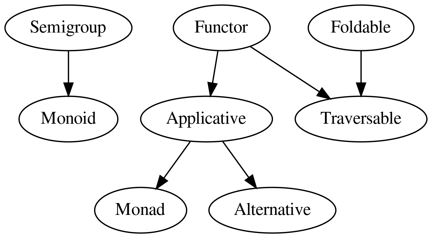 { width=500px }
Instance Search
Whenever a typeclass method is invoked at a callsite, GHC will perform an instance search over all available instances defined for the given typeclass associated with the method. This instance search is quite similar to backward chaining in logic programming languages. The search is performed during compilation after all types in all modules are known and is performed globally across all modules and all packages available to be linked. The instance search can either result in no instances, a single instance or multiple instances which satisfy the conditions of the call site.
Orphan Instances
Normally typeclass definitions are restricted to be defined in one of two places:
- In the same module as the declaration of the datatype in the instance head.
- In the same module as the class declaration.
These two restrictions restrict the instance search space to a system where a solution (if it exists) can always be found. If we allowed instances to be defined in any modules then we could potentially have multiple class instances defined in multiple modules and the search would be ambiguous.
This restriction can however be disabled with the -fno-warn-orphans flag.
{-# OPTIONS_GHC -fno-warn-orphans #-}
This will allow you to define orphan instances in the current module. But beware this will make the instance search contingent on your import list and may result in clashes in your codebase where the linker will fail because there are multiple modules which define the same instance head.
When used appropriately this can be the way to route around the fact that upstream modules may define datatypes that you use, but they have not defined the instances for other downstream libraries that you also use. You can then write these instances for your codebase without modifying either upstream library.
Minimal Annotations
In the presence of default implementations for typeclass methods, there may be several ways to implement a typeclass. For instance Eq is entirely defined by either defining when two values are equal or not equal by implying taking the negation of the other. We can define equality in terms of non-equality and vice-versa.
class Eq a where
(==), (/=) :: a -> a -> Bool
x == y = not (x /= y)
x /= y = not (x == y)
Before 7.6.1 there was no way to specify what was the "minimal" definition required to implement a typeclass
class Eq a where
(==), (/=) :: a -> a -> Bool
x == y = not (x /= y)
x /= y = not (x == y)
{-# MINIMAL (==) #-}
{-# MINIMAL (/=) #-}
Minimal pragmas are boolean expressions. For instance, with | as logical
OR, either definition of the above functions must be defined. Comma
indicates logical AND where both definitions must be defined.
{-# MINIMAL (==) | (/=) #-} -- Either (==) or (/=)
{-# MINIMAL (==) , (/=) #-} -- Both (==) and (/=)
Compiling the -Wmissing-methods will warn when an instance is defined that
does not meet the minimal criterion.
TypeSynonymInstances
Normally type class definitions are restricted to being defined only over fully expanded types with all type synonym indirections removed. Type synonyms introduce a "naming indirection" that can be included in the instance search to allow you to write synonym instances for multiple synonyms which expand to concrete types.
This is used quite often in modern Haskell.
FlexibleInstances
Normally the head of a typeclass instance must contain only a type constructor
applied to any number of type variables. There can be no nesting of other
constructors or non-type variables in the head. The FlexibleInstances
extension loosens this restriction to allow arbitrary nesting and non-type
variables to be mentioned in the head definition. This extension also implicitly
enables TypeSynonymInstances.
FlexibleContexts
Just as with instances, contexts normally are also constrained to consist
entirely of constraints where a class is applied to just type variables. The
FlexibleContexts extension lifts this restriction and allows any type of type
variable and nesting to occur the class constraint head. There is however still a
global restriction that all class hierarchies must not contain cycles.
OverlappingInstances
Typeclasses are normally globally coherent, there is only ever one instance that can be resolved for a type unambiguously at any call site in the program. There are however extensions to loosen this restriction and perform more manual direction of the instance search.
Overlapping instances loosens the coherent condition (there can be multiple instances) but introduces a criterion that it will resolve to the most specific one.
Historically enabling on the module-level was not the best idea, since
generally we define multiple classes in a module only a subset of which may be
incoherent. As of GHC 7.10 we now have the capacity to just annotate instances
with the OVERLAPPING and INCOHERENT inline pragmas.
IncoherentInstances
Incoherent instances loosens the restriction that there be only one specific
instance, it will be chosen based on a more complex search procedure which tries to
identify a prime instance based on information incorporated form OVERLAPPING
pragmas on instances in the search tree. Unless one is doing very advanced
type-level programming use class constraints, this is usually a poor design
decision and a sign to rethink the class hierarchy.
An example with INCOHERENT annotations:
Laziness
Haskell is a unique language that explores an alternative evaluation model called lazy evaluation. Lazy evaluation implies that expressions will be evaluated only when needed. In truth, this evaluation may even be indefinitely deferred. Consider the example in Haskell of defining an infinite list:
λ> mkInfinite n = n : mkInfinite n
λ> take 5 $ mkInfinite 4
[4,4,4,4,4]
The primary advantage of lazy evaluation in the large is that algorithms that operate over both unbounded and bounded data structures can inhabit the same type signatures and be composed without any additional need to restructure their logic or force intermediate computations.
Still, it's important to recognize that this is another subject on which much ink has been spilled. In fact, there is an ongoing discussion in the land of Haskell about the compromises between lazy and strict evaluation, and there are nuanced arguments for having either paradigm be the default.
Haskell takes a hybrid approach where it allows strict evaluation when needed while it uses laziness by default. Needless to say, we can always find examples where strict evaluation exhibits worse behavior than lazy evaluation and vice versa. These days Haskell can be both as lazy or as strict as you like, giving you options for however you prefer to program.
Languages that attempt to bolt laziness on to a strict evaluation model often bifurcate classes of algorithms into ones that are hand-adjusted to consume unbounded structures and those which operate over bounded structures. In strict languages, mixing and matching between lazy vs. strict processing often necessitates manifesting large intermediate structures in memory when such composition would “just work” in a lazy language.
By virtue of Haskell being the only language to actually explore this point in the design space, knowledge about lazy evaluation is not widely absorbed into the collective programmer consciousness and can often be non-intuitive to the novice. Some time is often needed to fully grok how lazy evaluation works
Strictness
For a more strict definition of strictnees, consider that there are several evaluation models for the lambda calculus:
- Strict - Evaluation is said to be strict if all arguments are evaluated before the body of a function.
- Non-strict - Evaluation is non-strict if the arguments are not necessarily evaluated before entering the body of a function.
These ideas give rise to several models, Haskell itself uses the call-by-need model.
Model Strictness Description
Call-by-value Strict Arguments evaluated before function entered Call-by-name Non-strict Arguments passed unevaluated Call-by-need Non-strict Arguments passed unevaluated but an expression is only evaluated once
Seq and WHNF
On the subject of laziness and evaluation, we have names for how fully evaluated an expression is. A term is said to be in weak head normal-form if the outermost constructor or lambda expression cannot be reduced further. A term is said to be in normal form if it is fully evaluated and all sub-expressions and thunks contained within are evaluated.
-- In Normal Form
42
(2, "foo")
\x -> x + 1
-- Not in Normal Form
1 + 2
(\x -> x + 1) 2
"foo" ++ "bar"
(1 + 1, "foo")
-- In Weak Head Normal Form
(1 + 1, "foo")
\x -> 2 + 2
'f' : ("oo" ++ "bar")
-- Not In Weak Head Normal Form
1 + 1
(\x -> x + 1) 2
"foo" ++ "bar"
In Haskell, normal evaluation only occurs at the outer constructor of case-statements in Core. If we pattern match on a list, we don’t implicitly force all values in the list. An element in a data structure is only evaluated up to the outermost constructor. For example, to evaluate the length of a list we need only scrutinize the outer Cons constructors without regard for their inner values:
λ: length [undefined, 1]
2
λ: head [undefined, 1]
Prelude.undefined
λ: snd (undefined, 1)
1
λ: fst (undefined, 1)
Prelude.undefined
For example, in a lazy language the following program terminates even though it contains diverging terms.
In a strict language like OCaml (ignoring its suspensions for the moment), the same program diverges.
Thunks
In Haskell a thunk is created to stand for an unevaluated computation. Evaluation of a thunk is called forcing the thunk. The result is an update, a referentially transparent effect, which replaces the memory representation of the thunk with the computed value. The fundamental idea is that a thunk is only updated once (although it may be forced simultaneously in a multi-threaded environment) and its resulting value is shared when referenced subsequently.
The GHCi command :sprint can be used to introspect the state of unevaluated
thunks inside an expression without forcing evaluation. For instance:
λ: let a = [1..] :: [Integer]
λ: let b = map (+ 1) a
λ: :sprint a
a = _
λ: :sprint b
b = _
λ: a !! 4
5
λ: :sprint a
a = 1 : 2 : 3 : 4 : 5 : _
λ: b !! 10
12
λ: :sprint a
a = 1 : 2 : 3 : 4 : 5 : 6 : 7 : 8 : 9 : 10 : 11 : _
λ: :sprint b
b = _ : _ : _ : _ : _ : _ : _ : _ : _ : _ : 12 : _
While a thunk is being computed its memory representation is replaced with a special form known as blackhole which indicates that computation is ongoing and allows for a short circuit when a computation might depend on itself to complete.
The seq function introduces an artificial dependence on the evaluation of
order of two terms by requiring that the first argument be evaluated to WHNF
before the evaluation of the second. The implementation of the seq function is
an implementation detail of GHC.
seq :: a -> b -> b
⊥ `seq` a = ⊥
a `seq` b = b
For one example where laziness can bite you, the infamous foldl is well-known to leak space when used carelessly and without several compiler optimizations applied. The strict foldl' variant uses seq to overcome this.
foldl :: (a -> b -> a) -> a -> [b] -> a
foldl f z [] = z
foldl f z (x:xs) = foldl f (f z x) xs
foldl' :: (a -> b -> a) -> a -> [b] -> a
foldl' _ z [] = z
foldl' f z (x:xs) = let z' = f z x in z' `seq` foldl' f z' xs
In practice, a combination between the strictness analyzer and the inliner on
-O2 will ensure that the strict variant of foldl is used whenever the
function is inlinable at call site so manually using foldl' is most often
not required.
Of important note is that GHCi runs without any optimizations applied so the same program that performs poorly in GHCi may not have the same performance characteristics when compiled with GHC.
BangPatterns
The extension BangPatterns allows an alternative syntax to force arguments
to functions to be wrapped in seq. A bang operator on an argument forces its
evaluation to weak head normal form before performing the pattern match. This
can be used to keep specific arguments evaluated throughout recursion instead of
creating a giant chain of thunks.
{-# LANGUAGE BangPatterns #-}
sum :: Num a => [a] -> a
sum = go 0
where
go !acc (x:xs) = go (acc + x) xs
go acc [] = acc
This is desugared into code effectively equivalent to the following:
sum :: Num a => [a] -> a
sum = go 0
where
go acc _ | acc `seq` False = undefined
go acc (x:xs) = go (acc + x) xs
go acc [] = acc
Function application to seq'd arguments is common enough that it has a special operator.
($!) :: (a -> b) -> a -> b
f $! x = let !vx = x in f vx
StrictData
As of GHC 8.0 strictness annotations can be applied to all definitions in a module automatically. In previous versions to make definitions strict it was necessary to use explicit syntactic annotations at call sites.
Enabling StrictData makes constructor fields strict by default on any module where the pragma is enabled:
{-# LANGUAGE StrictData #-}
data Employee = Employee
{ name :: T.Text
, age :: Int
}
Is equivalent to:
data Employee = Employee
{ name :: !T.Text
, age :: !Int
}
Strict
Strict implies -XStrictData and extends strictness annotations to all
arguments of functions.
f x y = x + y
Is equivalent to the following function declaration with explicit bang patterns:
f !x !y = x + y
On a module-level this effectively makes Haskell a call-by-value language with some caveats. All arguments to functions are now explicitly evaluated and all data in constructors within this module are in head normal form by construction.
Deepseq
There are often times when for performance reasons we need to deeply evaluate a
data structure to normal form leaving no terms unevaluated. The deepseq
library performs this task.
The typeclass NFData (Normal Form Data) allows us to seq all elements of a
structure across any subtypes which themselves implement NFData.
class NFData a where
rnf :: a -> ()
rnf a = a `seq` ()
deepseq :: NFData a => a -> b -> b
($!!) :: (NFData a) => (a -> b) -> a -> b
instance NFData Int
instance NFData (a -> b)
instance NFData a => NFData (Maybe a) where
rnf Nothing = ()
rnf (Just x) = rnf x
instance NFData a => NFData [a] where
rnf [] = ()
rnf (x:xs) = rnf x `seq` rnf xs
[1, undefined] `seq` ()
-- ()
[1, undefined] `deepseq` ()
-- Prelude.undefined
To force a data structure itself to be fully evaluated we share the same argument in both positions of deepseq.
force :: NFData a => a -> a
force x = x `deepseq` x
Irrefutable Patterns
A lazy pattern doesn't require a match on the outer constructor, instead it lazily calls the accessors of the values as needed. In the presence of a bottom, we fail at the usage site instead of the outer pattern match.
The Debate
Laziness is a controversial design decision in Haskell. It is difficult to write production Haskell code that operates in constant memory without some insight into the evaluation model and the runtime. A lot of industrial codebases have a policy of marking all constructors as strict by default or enabling [StrictData] to prevent space leaks. If Haskell were being designed from scratch it probably would not choose laziness as the default model. Future implementations of Haskell compilers would not choose this point in the design space if given the option of breaking with the language specification.
There is a lot of fear, uncertainty and doubt spread about lazy evaluation that unfortunately loses the forest for the trees and ignores 30 years of advanced research on the type system. In industrial programming a lot of software is sold on the meme of being of fast instead of being correct, and lazy evaluation is an intellectually easy talking point about these upside-down priorities. Nevertheless the colloquial perception of laziness being "evil" is a meme that will continue to persist regardless of any underlying reality because software is intrinsically a social process.
Prelude
What to Avoid?
Haskell being a 30 year old language has witnessed several revolutions in the way we structure and compose functional programs. Yet as a result several portions of the Prelude still reflect old schools of thought that simply can't be removed without breaking significant parts of the ecosystem.
Currently it really only exists in folklore which parts to use and which not to use, although this is a topic that almost all introductory books don't mention and instead make extensive use of the Prelude for simplicity's sake.
The short version of the advice on the Prelude is:
The instances of Foldable for the list type often conflict with the monomorphic versions in the Prelude which are left in for historical reasons. So oftentimes it is desirable to explicitly mask these functions from implicit import and force the use of Foldable and Traversable instead.
Of course oftentimes one wishes to only use the Prelude explicitly and one can explicitly import it qualified and use the pieces as desired without the implicit import of the whole namespace.
import qualified Prelude as P
What Should be in Prelude
To get work done on industrial projects you probably need the following libraries:
textcontainersunordered-containersmtltransformersvectorfilepathdirectoryprocessbytestringoptparse-applicativeunixaeson
Custom Preludes
The default Prelude can be disabled in its entirety by twiddling the
-XNoImplicitPrelude flag which allows us to replace the default import
entirely with a custom prelude. Many industrial projects will roll their own
Prologue.hs module which replaces the legacy prelude.
{-# LANGUAGE NoImplicitPrelude #-}
For example if we wanted to build up a custom project prelude we could construct
a Prologue module and dump the relevant namespaces we want from base into our
custom export list. Using the module reexport feature allows us to create an
Exports namespace which contains our Prelude's symbols. Every subsequent
module in our project will then have import Prologue as the first import.
module Prologue (
module Exports,
) where
import Data.Int as Exports
import Data.Tuple as Exports
import Data.Maybe as Exports
import Data.String as Exports
import Data.Foldable as Exports
import Data.Traversable as Exports
import Control.Monad.Trans.Except
as Exports
(ExceptT(ExceptT), Except, except, runExcept, runExceptT,
mapExcept, mapExceptT, withExcept, withExceptT)
Preludes
There are many approaches to custom preludes. The most widely used ones are all available on Hackage.
Different preludes take different approaches to defining what the Haskell standard library should be. Some are interoperable with existing code and others require an "all-in" approach that creates an ecosystem around it. Some projects are more community efforts and others are developed by consulting companies or industrial users wishing to standardise their commercial code.
In Modern Haskell there are many different perspectives on Prelude design and the degree to which more advanced ideas should be used. Which one is right for you is a matter of personal preference and constraints in your company.
Protolude
Protolude is a minimalist Prelude which provides many sensible defaults for writing modern Haskell and is compatible with existing code.
{-# LANGUAGE NoImplicitPrelude #-}
import Protolude
Protolude is one of the more conservative preludes and is developed by the author of this document.
See:
Partial Functions
A partial function is a function which doesn't terminate and yield a value for all given inputs. Conversely a total function terminates and is always defined for all inputs. As mentioned previously, certain historical parts of the Prelude are full of partial functions.
The difference between partial and total functions is the compiler can't reason about the runtime safety of partial functions purely from the information specified in the language and as such the proof of safety is left to the user to guarantee. They are safe to use in the case where the user can guarantee that invalid inputs cannot occur, but like any unchecked property its safety or not-safety is going to depend on the diligence of the programmer. This very much goes against the overall philosophy of Haskell and as such they are discouraged when not necessary.
head :: [a] -> a
read :: Read a => String -> a
(!!) :: [a] -> Int -> a
A list of partial functions in the default prelude:
Partial for all inputs
errorundefinedfail-- ForMonad IO
Partial for empty lists
headinittaillastfoldr1foldl1cyclemaximumminimum
Partial for Nothing
fromJust
Partial for invalid strings lists
read
Partial for infinite lists
sumproductreverse
Partial for negative or unbounded numbers
(!)(!!)toEnumgenericIndex
Replacing Partiality
The Prelude has total variants of the historical partial functions (e.g. Text.Read.readMaybe) in some
cases, but often these are found in the various replacement preludes
The total versions provided fall into three cases:
May- return Nothing when the function is not defined for the inputsDef- provide a default value when the function is not defined for the inputsNote- callerrorwith a custom error message when the function is not defined for the inputs. This is not safe, but slightly easier to debug!
-- Total
headMay :: [a] -> Maybe a
readMay :: Read a => String -> Maybe a
atMay :: [a] -> Int -> Maybe a
-- Total
headDef :: a -> [a] -> a
readDef :: Read a => a -> String -> a
atDef :: a -> [a] -> Int -> a
-- Partial
headNote :: String -> [a] -> a
readNote :: Read a => String -> String -> a
atNote :: String -> [a] -> Int -> a
Boolean Blindness
Boolean blindness is a common problem found in many programming languages. Consider the following two definitions which deconstruct a Maybe value into a boolean. Is there anything wrong with the definitions and below and why is this not caught in the type system?
data Bool = True | False
isNotJust :: Maybe a -> Bool
isNotJust (Just x) = True -- ???
isNotJust Nothing = False
isJust :: Maybe a -> Bool
isJust (Just x) = True
isJust Nothing = False
The problem with the Bool type is that there is effectively no difference
between True and False at the type level. A proposition taking a value to a Bool
takes any information given and destroys it. To reason about the behavior we
have to trace the provenance of the proposition we're getting the boolean answer
from, and this introduces a whole slew of possibilities for misinterpretation.
In the worst case, the only way to reason about safe and unsafe use of a
function is by trusting that a predicate's lexical name reflects its provenance!
For instance, testing some proposition over a Bool value representing whether the branch can perform the computation safely in the presence of a null is subject to accidental interchange. Consider that in a language like C or Python testing whether a value is null is indistinguishable to the language from testing whether the value is not null. Which of these programs encodes safe usage and which segfaults?
# This one?
if p(x):
# use x
elif not p(x):
# don't use x
# Or this one?
if p(x):
# don't use x
elif not p(x):
# use x
From inspection we can't tell without knowing how p is defined, the compiler can't distinguish the two either and thus the language won't save us if we happen to mix them up. Instead of making invalid states unrepresentable we've made the invalid state indistinguishable from the valid one!
The more desirable practice is to match on terms which explicitly witness the proposition as a type (often in a sum type) and won't typecheck otherwise.
case x of
Just a -> use x
Nothing -> don't use x
-- not ideal
case p x of
True -> use x
False -> don't use x
-- not ideal
if p x
then use x
else don't use x
To be fair though, many popular languages completely lack the notion of sum types (the source of many woes in my opinion) and only have product types, so this type of reasoning sometimes has no direct equivalence for those not familiar with ML family languages.
In Haskell, the Prelude provides functions like isJust and fromJust both of which can be used to
subvert this kind of reasoning and make it easy to introduce bugs and should often be avoided.
Foldable / Traversable
If coming from an imperative background retraining oneself to think about iteration over lists in terms of maps, folds, and scans can be challenging.
Prelude.foldl :: (a -> b -> a) -> a -> [b] -> a
Prelude.foldr :: (a -> b -> b) -> b -> [a] -> b
-- pseudocode
foldr f z [a...] = f a (f b ( ... (f y z) ... ))
foldl f z [a...] = f ... (f (f z a) b) ... y
For a concrete example consider the simple arithmetic sequence over the binary operator
(+):
-- foldr (+) 1 [2..]
(2 + (3 + (4 + (5 + ...))))
-- foldl (+) 1 [2..]
((((1 + 2) + 3) + 4) + ...)
Foldable and Traversable are the general interface for all traversals and folds of any data structure which is parameterized over its element type ( List, Map, Set, Maybe, ...). These two classes are used everywhere in modern Haskell and are extremely important.
class Foldable t where
fold :: Monoid m => t m -> m
foldMap :: Monoid m => (a -> m) -> t a -> m
foldr :: (a -> b -> b) -> b -> t a -> b
foldr' :: (a -> b -> b) -> b -> t a -> b
foldl :: (b -> a -> b) -> b -> t a -> b
foldl' :: (b -> a -> b) -> b -> t a -> b
foldr1 :: (a -> a -> a) -> t a -> a
foldl1 :: (a -> a -> a) -> t a -> a
toList :: t a -> [a]
null :: t a -> Bool
length :: t a -> Int
elem :: Eq a => a -> t a -> Bool
maximum :: Ord a => t a -> a
minimum :: Ord a => t a -> a
sum :: Num a => t a -> a
product :: Num a => t a -> a
A foldable instance allows us to apply functions to data types of monoidal
values that collapse the structure using some logic over mappend.
A traversable instance allows us to apply functions to data types that walk the structure left-to-right within an applicative context.
class (Functor f, Foldable f) => Traversable f where
traverse :: Applicative g => (a -> g b) -> f a -> g (f b)
class Foldable f where
foldMap :: Monoid m => (a -> m) -> f a -> m
The foldMap function is extremely general and non-intuitively many of the
monomorphic list folds can themselves be written in terms of this single
polymorphic function.
foldMap takes a function of values to a monoidal quantity, a functor over
the values and collapses the functor into the monoid. For instance for the
trivial Sum monoid:
λ: foldMap Sum [1..10]
Sum {getSum = 55}
For instance if we wanted to map a list of some abstract element types into a hashtable of elements based on pattern matching we could use it.
import Data.Foldable
import qualified Data.Map as Map
data Elt
= Elt Int Double
| Nil
foo :: [Elt] -> Map.Map Int Double
foo = foldMap go
where
go (Elt x y) = Map.singleton x y
go Nil = Map.empty
The full Foldable class (with all default implementations) contains a variety of
derived functions which themselves can be written in terms of foldMap and
Endo.
newtype Endo a = Endo {appEndo :: a -> a}
instance Monoid (Endo a) where
mempty = Endo id
Endo f `mappend` Endo g = Endo (f . g)
For example:
foldr :: (a -> b -> b) -> b -> t a -> b
foldr f z t = appEndo (foldMap (Endo . f) t) z
Most of the operations over lists can be generalized in terms of combinations of Foldable and Traversable to derive more general functions that work over all data structures implementing Foldable.
Data.Foldable.elem :: (Eq a, Foldable t) => a -> t a -> Bool
Data.Foldable.sum :: (Num a, Foldable t) => t a -> a
Data.Foldable.minimum :: (Ord a, Foldable t) => t a -> a
Data.Traversable.mapM :: (Monad m, Traversable t) => (a -> m b) -> t a -> m (t b)
Unfortunately for historical reasons the names exported by Foldable quite often conflict with ones defined in the Prelude, either import them qualified or just disable the Prelude. The operations in the Foldable class all specialize to the same and behave the same as the ones in Prelude for List types.
The instances we defined above can also be automatically derived by GHC using several language extensions. The automatic instances are identical to the hand-written versions above.
{-# LANGUAGE DeriveFunctor #-}
{-# LANGUAGE DeriveFoldable #-}
{-# LANGUAGE DeriveTraversable #-}
data Tree a = Node a [Tree a]
deriving (Show, Functor, Foldable, Traversable)
Strings
The string situation in Haskell is a sad affair. The default String type is defined as linked list of pointers to characters which is an extremely pathological and inefficient way of representing textual data. Unfortunately for historical reasons large portions of GHC and Base depend on String.
The String problem is intrinsically linked to the fact that the default GHC
Prelude provides a set of broken defaults that are difficult to change because
GHC and the entire ecosystem historically depend on it. There are however high
performance string libraries that can swapped in for the broken String type
and we will discuss some ways of working with high-performance and memory
efficient replacements.
String
The default Haskell string type is implemented as a naive linked list of characters, this is hilariously terrible for most purposes but no one knows how to fix it without rewriting large portions of all code that exists, and simply nobody wants to commit the time to fix it. So it remains broken, likely forever.
type String = [Char]
However, fear not as there are are two replacement libraries for processing
textual data: text and bytestring.
text- Used for handling unicode data.bytestring- Used for handling ASCII data that needs to interchange with C code or network protocols.
For each of these there are two variants for both text and bytestring.
- lazy - Lazy text objects are encoded as lazy lists of strict chunks of bytes.
- strict - Byte vectors are encoded as strict Word8 arrays of bytes or code points
Giving rise to the Cartesian product of the four common string types:
Variant Module
strict text Data.Text
lazy text Data.Text.Lazy
strict bytestring Data.ByteString
lazy bytestring Data.ByteString.Lazy
String Conversions
Conversions between strings types are done with several functions across the bytestring and text libraries. The mapping between text and bytestring is inherently lossy so there is some degree of freedom in choosing the encoding. We'll just consider utf-8 for simplicity.
Data.Text Data.Text.Lazy Data.ByteString Data.ByteString.Lazy
Data.Text id fromStrict encodeUtf8 encodeUtf8 Data.Text.Lazy toStrict id encodeUtf8 encodeUtf8 Data.ByteString decodeUtf8 decodeUtf8 id fromStrict Data.ByteString.Lazy decodeUtf8 decodeUtf8 toStrict id
Table: From : left column, To : top row
Be careful with the functions (decodeUtf8, decodeUtf16LE, etc.) as they are
partial and will throw errors if the byte array given does not contain unicode
code points. Instead use one of the following functions which will allow you to
explicitly handle the error case:
decodeUtf8' :: ByteString -> Either UnicodeException Text
decodeUtf8With :: OnDecodeError -> ByteString -> Text
OverloadedStrings
With the -XOverloadedStrings extension string literals can be overloaded
without the need for explicit packing and can be written as string literals in
the Haskell source and overloaded via the typeclass IsString. Sometimes this
is desirable.
class IsString a where
fromString :: String -> a
For instance:
λ: :type "foo"
"foo" :: [Char]
λ: :set -XOverloadedStrings
λ: :type "foo"
"foo" :: IsString a => a
We can also derive IsString for newtypes using GeneralizedNewtypeDeriving,
although much of the safety of the newtype is then lost if it is used interchangeable
with other strings.
newtype Cat = Cat Text
deriving (IsString)
fluffy :: Cat
fluffy = "Fluffy"
Import Conventions
Since there are so many modules that provide string datatypes, and these modules are used ubiquitously, some conventions are often adopted to import these modules as specific agreed-upon qualified names. In many Haskell projects you will see the following social conventions used for distinguish text types.
For datatypes:
import qualified Data.Text as T
import qualified Data.Text.Lazy as TL
import qualified Data.ByteString as BS
import qualified Data.ByteString.Lazy as BL
import qualified Data.ByteString.Char8 as C
import qualified Data.ByteString.Lazy.Char8 as CL
For IO operations:
import qualified Data.Text.IO as TIO
import qualified Data.Text.Lazy.IO as TLIO
For encoding operations:
import qualified Data.Text.Encoding as TE
import qualified Data.Text.Lazy.Encoding as TLE
In addition many libraries and alternative preludes will define the following type synonyms:
type LText = TL.Text
type LByteString = BL.ByteString
Text
The Text type is a packed blob of Unicode characters.
pack :: String -> Text
unpack :: Text -> String
See: Text
Text.Builder
toLazyText :: Builder -> Data.Text.Lazy.Internal.Text
fromLazyText :: Data.Text.Lazy.Internal.Text -> Builder
The Text.Builder allows the efficient monoidal construction of lazy Text types without having to go through inefficient forms like String or List types as intermediates.
ByteString
ByteStrings are arrays of unboxed characters with either strict or lazy evaluation.
pack :: String -> ByteString
unpack :: ByteString -> String
Printf
Haskell also has a variadic printf function in the style of C.
Overloaded Lists
It is ubiquitous for data structure libraries to expose toList and fromList functions to construct
various structures out of lists. As of GHC 7.8 we now have the ability to overload the list syntax in the
surface language with the typeclass IsList.
class IsList l where
type Item l
fromList :: [Item l] -> l
fromListN :: Int -> [Item l] -> l
toList :: l -> [Item l]
instance IsList [a] where
type Item [a] = a
fromList = id
toList = id
λ: :seti -XOverloadedLists
λ: :type [1,2,3]
[1,2,3] :: (Num (GHC.Exts.Item l), GHC.Exts.IsList l) => l
For example we could write an overloaded list instance for hash tables that
simply converts to the hash table using fromList. Some math libraries that
use vector-like structures will use overloaded lists in this fashion.
Regex
regex-tdfa implements POSIX extended regular expressions. These can operate
over any of the major string types and with OverloadedStrings enabled allows you
to write well-typed regex expressions as strings.
Escaping Text
Haskell uses C-style single-character escape codes
Escape Unicode Character
\n U+000A newline \0 U+0000 null character \& n/a empty string \' U+0027 single quote \\ U+005C backslash \a U+0007 alert \b U+0008 backspace \f U+000C form feed \r U+000D carriage return \t U+0009 horizontal tab \v U+000B vertical tab \" U+0022 double quote
String Splitting
The split package provides a variety of missing functions for splitting list and string types.
Applicatives
Like monads Applicatives are an abstract structure for a wide class of computations that sit between functors and monads in terms of generality.
pure :: Applicative f => a -> f a
(<$>) :: Functor f => (a -> b) -> f a -> f b
(<*>) :: f (a -> b) -> f a -> f b
As of GHC 7.6, Applicative is defined as:
class Functor f => Applicative f where
pure :: a -> f a
(<*>) :: f (a -> b) -> f a -> f b
(<$>) :: Functor f => (a -> b) -> f a -> f b
(<$>) = fmap
With the following laws:
pure id <*> v = v
pure f <*> pure x = pure (f x)
u <*> pure y = pure ($ y) <*> u
u <*> (v <*> w) = pure (.) <*> u <*> v <*> w
As an example, consider the instance for Maybe:
instance Applicative Maybe where
pure = Just
Nothing <*> _ = Nothing
_ <*> Nothing = Nothing
Just f <*> Just x = Just (f x)
As a rule of thumb, whenever we would use m >>= return . f what we probably want is an applicative
functor, and not a monad.
The pattern f <$> a <*> b ... shows up so frequently that there is a family
of functions to lift applicatives of a fixed number arguments. This pattern
also shows up frequently with monads (liftM, liftM2, liftM3).
liftA :: Applicative f => (a -> b) -> f a -> f b
liftA f a = pure f <*> a
liftA2 :: Applicative f => (a -> b -> c) -> f a -> f b -> f c
liftA2 f a b = f <$> a <*> b
liftA3 :: Applicative f => (a -> b -> c -> d) -> f a -> f b -> f c -> f d
liftA3 f a b c = f <$> a <*> b <*> c
Applicative also has functions *> and <* that sequence applicative
actions while discarding the value of one of the arguments. The operator *>
discards the left while <* discards the right. For example in a monadic
parser combinator library the *> would parse with first parser argument but
return the second.
The Applicative functions <$> and <*> are generalized by liftM and
ap for monads.
import Control.Monad
import Control.Applicative
data C a b = C a b
mnd :: Monad m => m a -> m b -> m (C a b)
mnd a b = C `liftM` a `ap` b
apl :: Applicative f => f a -> f b -> f (C a b)
apl a b = C <$> a <*> b
See: Applicative Programming with Effects
Alternative
Alternative is an extension of the Applicative class with a zero element and an associative binary operation respecting the zero.
class Applicative f => Alternative f where
-- | The identity of '<|>'
empty :: f a
-- | An associative binary operation
(<|>) :: f a -> f a -> f a
-- | One or more.
some :: f a -> f [a]
-- | Zero or more.
many :: f a -> f [a]
optional :: Alternative f => f a -> f (Maybe a)
when :: (Alternative f) => Bool -> f () -> f ()
when p s = if p then s else return ()
guard :: (Alternative f) => Bool -> f ()
guard True = pure ()
guard False = mzero
instance Alternative Maybe where
empty = Nothing
Nothing <|> r = r
l <|> _ = l
instance Alternative [] where
empty = []
(<|>) = (++)
λ: foldl1 (<|>) [Nothing, Just 5, Just 3]
Just 5
These instances show up very frequently in parsers where the alternative operator can model alternative parse branches.
Arrows
A category is an algebraic structure that includes a notion of an identity and a composition operation that is associative and preserves identities. In practice arrows are not often used in modern Haskell and are often considered a code smell.
class Category cat where
id :: cat a a
(.) :: cat b c -> cat a b -> cat a c
instance Category (->) where
id = Prelude.id
(.) = (Prelude..)
(<<<) :: Category cat => cat b c -> cat a b -> cat a c
(<<<) = (.)
(>>>) :: Category cat => cat a b -> cat b c -> cat a c
f >>> g = g . f
Arrows are an extension of categories with the notion of products.
class Category a => Arrow a where
arr :: (b -> c) -> a b c
first :: a b c -> a (b,d) (c,d)
second :: a b c -> a (d,b) (d,c)
(***) :: a b c -> a b' c' -> a (b,b') (c,c')
(&&&) :: a b c -> a b c' -> a b (c,c')
The canonical example is for functions.
instance Arrow (->) where
arr f = f
first f = f *** id
second f = id *** f
(***) f g ~(x,y) = (f x, g y)
In this form, functions of multiple arguments can be threaded around using the arrow combinators in a much more pointfree form. For instance a histogram function has a nice one-liner.
import Data.List (group, sort)
histogram :: Ord a => [a] -> [(a, Int)]
histogram = map (head &&& length) . group . sort
λ: histogram "Hello world"
[(' ',1),('H',1),('d',1),('e',1),('l',3),('o',2),('r',1),('w',1)]
Arrow notation
GHC has builtin syntax for composing arrows using proc notation. The
following are equivalent after desugaring:
{-# LANGUAGE Arrows #-}
addA :: Arrow a => a b Int -> a b Int -> a b Int
addA f g = proc x -> do
y <- f -< x
z <- g -< x
returnA -< y + z
addA f g = arr (\ x -> (x, x)) >>>
first f >>> arr (\ (y, x) -> (x, y)) >>>
first g >>> arr (\ (z, y) -> y + z)
addA f g = f &&& g >>> arr (\ (y, z) -> y + z)
In practice this notation is not often used and may become deprecated in the future.
See: Arrow Notation
Bifunctors
Bifunctors are a generalization of functors to include types parameterized by two parameters and include two map functions for each parameter.
class Bifunctor p where
bimap :: (a -> b) -> (c -> d) -> p a c -> p b d
first :: (a -> b) -> p a c -> p b c
second :: (b -> c) -> p a b -> p a c
The bifunctor laws are a natural generalization of the usual functor laws. Namely they respect identities and composition in the usual way:
bimap id id ≡ id
first id ≡ id
second id ≡ id
bimap f g ≡ first f . second g
The canonical example is for 2-tuples.
λ: first (+1) (1,2)
(2,2)
λ: second (+1) (1,2)
(1,3)
λ: bimap (+1) (+1) (1,2)
(2,3)
λ: first (+1) (Left 3)
Left 4
λ: second (+1) (Left 3)
Left 3
λ: second (+1) (Right 3)
Right 4
Polyvariadic Functions
One surprising application of typeclasses is the ability to construct functions which take an arbitrary number of arguments by defining instances over function types. The arguments may be of arbitrary type, but the resulting collected arguments must either be converted into a single type or unpacked into a sum type.
Error Handling
There are a plethora of ways of handling errors in Haskell. While Haskell's runtime supports throwing and handling exceptions, it is important to use the right method in the right context.
Either Monad
In keeping with the Haskell tradition it is always preferable to use pure logic
when possible. In many simple cases error handling can be done quite simply by
using the Monad instance of Either. Monadic bind simply threads a Right
value through the monad and "short-circuits" evaluation when a Left is
introduced. This is simple enough error handling which privileges the Left
constructor to hold the error. Many simple functions which can fail can simply
use the Either Error a in the result type to encode simple error handling.
The downside to this is that it forces every consumer of the function to pattern
match on the result to handle the error case. It also assumes that all Error
types can be encoded inside of the sum type holding the possible failures.
saveDiv -> Float -> Float -> Either DivError Float
safeDiv x 0 = Left NoDivZero
safeDiv x y = Right (x `div` y)
ExceptT
When using the transformers style effect stacks it is quite common to need to have
a layer of the stack which can fail. When using the style of composing effects a
monad transformer (which is a wrapper around Either monad) can be added which
lifts the error handling into an ExceptT effect layer.
As of mtl 2.2 or higher, the ErrorT class has been replaced by
ExceptT at the transformers level.
newtype ExceptT e m a = ExceptT (m (Either e a))
runExceptT :: ExceptT e m a -> m (Either e a)
runExceptT (ExceptT m) = m
instance (Monad m) => Monad (ExceptT e m) where
return a = ExceptT $ return (Right a)
m >>= k = ExceptT $ do
a <- runExceptT m
case a of
Left e -> return (Left e)
Right x -> runExceptT (k x)
fail = ExceptT . fail
throwE :: (Monad m) => e -> ExceptT e m a
throwE = ExceptT . return . Left
catchE :: (Monad m) =>
ExceptT e m a -- ^ the inner computation
-> (e -> ExceptT e' m a) -- ^ a handler for exceptions in the inner
-- computation
-> ExceptT e' m a
m `catchE` h = ExceptT $ do
a <- runExceptT m
case a of
Left l -> runExceptT (h l)
Right r -> return (Right r)
And also this can be extended to the mtl MonadError instance for which we can
write instances for IO and Either themselves:
instance MonadTrans (ExceptT e) where
lift = ExceptT . liftM Right
class (Monad m) => MonadError e m | m -> e where
throwError :: e -> m a
catchError :: m a -> (e -> m a) -> m a
instance MonadError IOException IO where
throwError = ioError
catchError = catch
instance MonadError e (Either e) where
throwError = Left
Left l `catchError` h = h l
Right r `catchError` _ = Right r
See:
Control.Exception
GHC has a builtin system for propagating errors up at the runtime level, below
the business logic level. These are used internally for all sorts of concurrency
and system interfaces. The runtime provides builtin operations throw and
catch functions which allow us to throw exceptions in pure code and catch
the resulting exception within IO. Note that the return value of throw
inhabits all types.
throw :: Exception e => e -> a
catch :: Exception e => IO a -> (e -> IO a) -> IO a
try :: Exception e => IO a -> IO (Either e a)
evaluate :: a -> IO a
Because a value will not be evaluated unless needed, if one desires to know for
sure that an exception is either caught or not it can be deeply forced into head
normal form before invoking catch. The strictCatch is not provided by
the standard library but has a simple implementation in terms of deepseq.
strictCatch :: (NFData a, Exception e) => IO a -> (e -> IO a) -> IO a
strictCatch = catch . (toNF =<<)
Exceptions
The problem with the previous approach is having to rely on GHC's asynchronous exception handling inside of IO
to handle basic operations and the bifurcation of APIs which need to expose
different APIs for any monad that has failure (IO, STM, ExceptT, etc.).
The exceptions package provides the same API as
Control.Exception but loosens the dependency on IO. It instead provides a
granular set of typeclasses which can operate over different monads which
require a precise subset of error handling methods.
MonadThrow- Monads which expose an interface for throwing exceptions.MonadCatch- Monads which expose an interface for handling exceptions.MonadMask- Monads which expose an interface for masking asynchronous exceptions.
There are three core primitives that are used in handling runtime exceptions:
finally- For handling guaranteed finalisation of code in the presence of exceptions.onException- For handing exception case only if an exception is thrown.bracket- For implementing resource handling with custom acquisition and finalizer logic, in the presence of exceptions.
finally takes an IO action to run as a computation and a secondary function
to run after the evaluation of the first.
finally :: IO a -- ^ computation to run first
-> IO b -- ^ computation to run afterward (even if an exception was raised)
-> IO a -- returns the value from the first computation
onException has a similar signature but the second function is run only if
an exception is raised.
onException :: IO a -> IO b -> IO a
The bracket function takes two functions, an acquisition function and a
finalizer function which "bracket" the evaluation of the third. The finaliser
will be run if the computation throwns an exception and unwinds.
bracket
:: IO a -- ^ computation to run first
-> (a -> IO b) -- ^ computation to run last
-> (a -> IO c) -- ^ computation to run in-between
-> IO c -- returns the value from the in-between computation
A simple example of usage is bracket logic that handles file descriptors which
need to be explicitly closed after evaluation is done. The initialiser in this
case will return a file descriptor to the body and then run hClose on the file
descriptor after the body is done with evaluation.
bracket
(openFile "myfile" ReadMode) -- acquisition
(hClose) -- finaliser
(\fileHandle -> ... ) -- body
In addition the exceptions library exposes several functions for explicitly
handling a variety of exceptions of various forms. Toplevel handlers that need
to "catch em' all" should use catchAny for wildcard error handling.
catch :: (MonadCatch m, Exception e) => m a -> (e -> m a) -> m a
catchIO :: MonadCatch m => m a -> (IOException -> m a) -> m a
catchAny :: MonadCatch m => m a -> (SomeException -> m a) -> m a
catchAsync :: (MonadCatch m, Exception e) => m a -> (e -> m a) -> m a
A simple example of usage:
See: exceptions
Spoon
Sometimes you'll be forced to deal with seemingly pure functions that can throw
up at any point. There are many functions in the standard library like this, and
many more on Hackage. You'd like to handle this logic purely as if it were
returning a proper Maybe a but to catch the logic you'd need to install an IO
handler inside IO to catch it. Spoon allows us to safely (and "purely", although
it uses a referentially transparent invocation of unsafePerformIO) to catch
these exceptions and put them in Maybe where they belong.
The spoon function evaluates its argument to head normal form, while
teaspoon evaluates to weak head normal form.
Advanced Monads
When working with the wider library you will find there a variety of "advanced monads" which are higher-level constructions on top of of the monadic interface which enrich the structure with additional rules or build APIs for combining different types of monads. Some of the most-used cases are mentioned in this section.
Function Monad
If one writes Haskell long enough one might eventually encounter the curious beast that is the ((->) r)
monad instance. It generally tends to be non-intuitive to work with, but is quite simple when one considers it
as an unwrapped Reader monad.
instance Functor ((->) r) where
fmap = (.)
instance Monad ((->) r) where
return = const
f >>= k = \r -> k (f r) r
This just uses a prefix form of the arrow type operator.
type Reader r = (->) r -- pseudocode
instance Monad (Reader r) where
return a = \_ -> a
f >>= k = \r -> k (f r) r
ask' :: r -> r
ask' = id
asks' :: (r -> a) -> (r -> a)
asks' f = id . f
runReader' :: (r -> a) -> r -> a
runReader' = id
RWS Monad
The RWS monad combines the functionality of the three monads discussed above, the Reader, Writer,
and State. There is also a RWST transformer.
runReader :: Reader r a -> r -> a
runWriter :: Writer w a -> (a, w)
runState :: State s a -> s -> (a, s)
These three eval functions are now combined into the following functions:
runRWS :: RWS r w s a -> r -> s -> (a, s, w)
execRWS :: RWS r w s a -> r -> s -> (s, w)
evalRWS :: RWS r w s a -> r -> s -> (a, w)
The usual caveat about Writer laziness also applies to RWS.
Cont
runCont :: Cont r a -> (a -> r) -> r
callCC :: MonadCont m => ((a -> m b) -> m a) -> m a
cont :: ((a -> r) -> r) -> Cont r a
In continuation passing style, composite computations are built up from sequences of nested computations which are terminated by a final continuation which yields the result of the full computation by passing a function into the continuation chain.
add :: Int -> Int -> Int
add x y = x + y
add :: Int -> Int -> (Int -> r) -> r
add x y k = k (x + y)
MonadPlus
Choice and failure.
class (Alternative m, Monad m) => MonadPlus m where
mzero :: m a
mplus :: m a -> m a -> m a
instance MonadPlus [] where
mzero = []
mplus = (++)
instance MonadPlus Maybe where
mzero = Nothing
Nothing `mplus` ys = ys
xs `mplus` _ys = xs
MonadPlus forms a monoid with
mzero `mplus` a = a
a `mplus` mzero = a
(a `mplus` b) `mplus` c = a `mplus` (b `mplus` c)
asum :: (Foldable t, Alternative f) => t (f a) -> f a
asum = foldr (<|>) empty
msum :: (Foldable t, MonadPlus m) => t (m a) -> m a
msum = asum
MonadFail
Before the great awakening, Monads used to be defined as the following class.
class Monad m where
(>>=) :: m a -> (a -> m b) -> m b
(>>) :: m a -> m b -> m b
return :: a -> m a
fail :: String -> m a
m >> k = m >>= \_ -> k
fail s = error s
This was eventually deemed not to be an great design and in particular the
fail function was a misplaced lawless entity that would generate bottoms. It
was also necessary to define fail for all monads, even those without a notion
of failure. This was considered quite ugly and eventually a breaking change to
base (landed in 4.9) was added which split out MonadFail into a separate class
where it belonged.
class Monad m => MonadFail m where
fail :: String -> m a
Some of the common instances of MonadFail are shown below:
instance MonadFail Maybe where
fail _ = Nothing
instance MonadFail [] where
{-# INLINE fail #-}
fail _ = []
instance MonadFail IO where
fail = failIO
MonadFix
The fixed point of a monadic computation. mfix f executes the action f only once, with the eventual
output fed back as the input.
fix :: (a -> a) -> a
fix f = let x = f x in x
mfix :: (a -> m a) -> m a
class Monad m => MonadFix m where
mfix :: (a -> m a) -> m a
instance MonadFix Maybe where
mfix f = let a = f (unJust a) in a
where unJust (Just x) = x
unJust Nothing = error "mfix Maybe: Nothing"
The regular do-notation can also be extended with -XRecursiveDo to accommodate recursive monadic bindings.
ST Monad
The ST monad models "threads" of stateful computations which can manipulate mutable references but are
restricted to only return pure values when evaluated and are statically confined to the ST monad of a s
thread.
runST :: (forall s. ST s a) -> a
newSTRef :: a -> ST s (STRef s a)
readSTRef :: STRef s a -> ST s a
writeSTRef :: STRef s a -> a -> ST s ()
Using the ST monad we can create a class of efficient purely functional data structures that use mutable references in a referentially transparent way.
Free Monads
Pure :: a -> Free f a
Free :: f (Free f a) -> Free f a
liftF :: (Functor f, MonadFree f m) => f a -> m a
retract :: Monad f => Free f a -> f a
Free monads are monads which instead of having a join operation that combines computations, instead forms
composite computations from application of a functor.
join :: Monad m => m (m a) -> m a
wrap :: MonadFree f m => f (m a) -> m a
One of the best examples is the Partiality monad which models computations which can diverge. Haskell allows
unbounded recursion, but for example we can create a free monad from the Maybe functor which can be
used to fix the call-depth of, for example the Ackermann function.
The other common use for free monads is to build embedded domain-specific languages to describe computations. We can model a subset of the IO monad by building up a pure description of the computation inside of the IOFree monad and then using the free monad to encode the translation to an effectful IO computation.
An implementation such as the one found in free might look like the following:
Indexed Monads
Indexed monads are a generalisation of monads that adds an additional type parameter to the class that carries information about the computation or structure of the monadic implementation.
class IxMonad md where
return :: a -> md i i a
(>>=) :: md i m a -> (a -> md m o b) -> md i o b
The canonical use-case is a variant of the vanilla State which allows type-changing on the state for intermediate steps inside of the monad. This indeed turns out to be very useful for handling a class of problems involving resource management since the extra index parameter gives us space to statically enforce the sequence of monadic actions by allowing and restricting certain state transitions on the index parameter at compile-time.
To make this more usable we'll use the somewhat esoteric -XRebindableSyntax allowing us to overload the
do-notation and if-then-else syntax by providing alternative definitions local to the module.
Lifted Base
The default prelude predates a lot of the work on monad transformers and as such
many of the common functions for handling errors and interacting with IO are
bound strictly to the IO monad and not to functions implementing stacks on top
of IO or ST. The lifted-base provides generic control operations such as
catch can be lifted from IO or any other base monad.
monad-base
Monad base provides an abstraction over liftIO and other functions to
explicitly lift into a "privileged" layer of the transformer stack. It's
implemented as a multiparameter typeclass with the "base" monad as the parameter b.
-- | Lift a computation from the base monad
class (Applicative b, Applicative m, Monad b, Monad m)
=> MonadBase b m | m -> b where
liftBase ∷ b a -> m a
monad-control
Monad control builds on top of monad-base to extended lifting operation to
control operations like catch and bracket can be written generically in
terms of any transformer with a base layer supporting these operations. Generic
operations can then be expressed in terms of a MonadBaseControl and written
in terms of the combinator control which handles the bracket and automatic
handler lifting.
control :: MonadBaseControl b m => (RunInBase m b -> b (StM m a)) -> m a
For example the function catch provided by Control.Exception is normally
locked into IO.
catch :: Exception e => IO a -> (e -> IO a) -> IO a
By composing it in terms of control we can construct a generic version which
automatically lifts inside of any combination of the usual transformer stacks
that has MonadBaseControl instance.
catch
:: (MonadBaseControl IO m, Exception e)
=> m a -- ^ Computation
-> (e -> m a) -- ^ Handler
-> m a
catch a handler = control $ \runInIO ->
E.catch (runInIO a)
(\e -> runInIO $ handler e)
Quantification
In logic a predicate is a statement about a subject. For instance the statement: Socrates is a man, can be written as:
Man(Socrates)
A predicate assigned to a variable Man(x) has a truth value if the predicate holds for the subject. The domain of a variable is the set of all variables that may be assigned to the variable. A quantifier turns predicates into propositions by assigning values to all variables. For example the statement: All men are mortal. This is an example of a universal quantifier which describe a predicate that holds forall inhabitants of the domain of variables.
Forall x. If Man(x) then Mortal(x)
The truth value that that Socrates is mortal can be derived from above relation. Programming with quantifiers in Haskell follows this same kind of logical convention except we will be working with types and constraints on types.
Universal Quantification
Universal quantification the primary mechanism of encoding polymorphism in
Haskell. The essence of universal quantification is that we can express
functions which operate the same way for a set of types and whose function
behavior is entirely determined only by the behavior of all types in this
span. These are represented at the type-level by in the introduction of a
universal quantifier (forall or ∀) over a set of the type variables in the
signature.
Normally quantifiers are omitted in type signatures since in Haskell's vanilla surface language it is unambiguous to assume to that free type variables are universally quantified. So the following two are equivalent:
id :: forall a. a -> a
id :: a -> a
Free Theorems
A universally quantified type-variable actually implies quite a few rather deep properties about the implementation of a function that can be deduced from its type signature. For instance the identity function in Haskell is guaranteed to only have one implementation since the only information that the information that can present in the body:
id :: forall a. a -> a
id x = x
These so called free theorems are properties that hold for any well-typed inhabitant of a universally quantified signature.
fmap :: Functor f => (a -> b) -> f a -> f b
For example a free theorem of fmap is that every implementation of functor
can only ever have the property that composition of maps of functions is the
same as maps of the functions composed together.
forall f g. fmap f . fmap g = fmap (f . g)
Type Systems
Hindley-Milner type system
The Hindley-Milner type system is historically important as one of the first typed lambda calculi that admitted both polymorphism and a variety of inference techniques that could always decide principal types.
e : x
| λx:t.e -- value abstraction
| e1 e2 -- application
| let x = e1 in e2 -- let
t : t -> t -- function types
| a -- type variables
σ : ∀ a . t -- type scheme
In an type checker implementation, a generalize function converts all type variables within the type into polymorphic type variables yielding a type scheme. While a instantiate function maps a scheme to a type, but with any polymorphic variables converted into unbound type variables.
Rank-N Types
System-F is the type system that underlies Haskell. System-F subsumes the HM type system in the sense that every type expressible in HM can be expressed within System-F. System-F is sometimes referred to in texts as the Girald-Reynolds polymorphic lambda calculus or second-order lambda calculus.
t : t -> t -- function types
| a -- type variables
| ∀ a . t -- forall
e : x -- variables
| λ(x:t).e -- value abstraction
| e1 e2 -- value application
| Λa.e -- type abstraction
| e_t -- type application
An example with equivalents of GHC Core in comments:
id : ∀ t. t -> t
id = Λt. λx:t. x
-- id :: forall t. t -> t
-- id = \ (@ t) (x :: t) -> x
tr : ∀ a. ∀ b. a -> b -> a
tr = Λa. Λb. λx:a. λy:b. x
-- tr :: forall a b. a -> b -> a
-- tr = \ (@ a) (@ b) (x :: a) (y :: b) -> x
fl : ∀ a. ∀ b. a -> b -> b
fl = Λa. Λb. λx:a. λy:b. y
-- fl :: forall a b. a -> b -> b
-- fl = \ (@ a) (@ b) (x :: a) (y :: b) -> y
nil : ∀ a. [a]
nil = Λa. Λb. λz:b. λf:(a -> b -> b). z
-- nil :: forall a. [a]
-- nil = \ (@ a) (@ b) (z :: b) (f :: a -> b -> b) -> z
cons : ∀ a. a -> [a] -> [a]
cons = Λa. λx:a. λxs:(∀ b. b -> (a -> b -> b) -> b).
Λb. λz:b. λf : (a -> b -> b). f x (xs_b z f)
-- cons :: forall a. a -> [a] -> [a]
-- cons = \ (@ a) (x :: a) (xs :: forall b. b -> (a -> b -> b) -> b)
-- (@ b) (z :: b) (f :: a -> b -> b) -> f x (xs @ b z f)
Normally when Haskell's typechecker infers a type signature it places all quantifiers of type variables at the outermost position such that no quantifiers appear within the body of the type expression, called the prenex restriction. This restricts an entire class of type signatures that would otherwise be expressible within System-F, but has the benefit of making inference much easier.
-XRankNTypes loosens the prenex restriction such that we may explicitly place quantifiers within the body
of the type. The bad news is that the general problem of inference in this relaxed system is undecidable in
general, so we're required to explicitly annotate functions which use RankNTypes or they are otherwise
inferred as rank 1 and may not typecheck at all.
Monomorphic Rank 0: t
Polymorphic Rank 1: forall a. a -> t
Polymorphic Rank 2: (forall a. a -> t) -> t
Polymorphic Rank 3: ((forall a. a -> t) -> t) -> t
Of important note is that the type variables bound by an explicit quantifier in a higher ranked type may not escape their enclosing scope. The typechecker will explicitly enforce this by enforcing that variables bound inside of rank-n types (called skolem constants) will not unify with free meta type variables inferred by the inference engine.
In this example in order for the expression to be well typed, f would
necessarily have (Int -> Int) which implies that a ~ Int over the whole
type, but since a is bound under the quantifier it must not be unified with
Int and so the typechecker must fail with a skolem capture error.
Couldn't match expected type `a' with actual type `t'
`a' is a rigid type variable bound by a type expected by the context: a -> a
`t' is a rigid type variable bound by the inferred type of g :: t -> Int
In the expression: x In the first argument of `escape', namely `(\ a -> x)'
In the expression: escape (\ a -> x)
This can actually be used for our advantage to enforce several types of
invariants about scope and use of specific type variables. For example the ST
monad uses a second rank type to prevent the capture of references between ST
monads with separate state threads where the s type variable is bound within
a rank-2 type and cannot escape, statically guaranteeing that the implementation
details of the ST internals can't leak out and thus ensuring its referential
transparency.
Existential Quantification
An existential type is a pair of a type and a term with a special set of packing and unpacking semantics. The type of the value encoded in the existential is known by the producer but not by the consumer of the existential value.
The existential over SBox gathers a collection of values defined purely in
terms of their Show interface and an opaque pointer, no other information is
available about the values and they can't be accessed or unpacked in any other
way.
Passing around existential types allows us to hide information from consumers of data types and restrict the behavior that functions can use. Passing records around with existential variables allows a type to be "bundled" with a fixed set of functions that operate over its hidden internals.
Impredicative Types
Although extremely brittle, GHC also has limited support for impredicative polymorphism which allows instantiating type variable with a polymorphic type. Implied is that this loosens the restriction that quantifiers must precede arrow types and now they may be placed inside of type-constructors.
-- Can't unify ( Int ~ Char )
revUni :: forall a. Maybe ([a] -> [a]) -> Maybe ([Int], [Char])
revUni (Just g) = Just (g [3], g "hello")
revUni Nothing = Nothing
Use of this extension is very rare, and there is some consideration that
-XImpredicativeTypes is fundamentally broken. Although GHC is very liberal
about telling us to enable it when one accidentally makes a typo in a type
signature!
Some notable trivia, the ($) operator is wired into GHC in a very special
way as to allow impredicative instantiation of runST to be applied via
($) by special-casing the ($) operator only when used for the ST monad.
For example if we define a function apply which should behave identically to
($) we'll get an error about polymorphic instantiation even though they are
defined identically!
{-# LANGUAGE RankNTypes #-}
import Control.Monad.ST
f `apply` x = f x
foo :: (forall s. ST s a) -> a
foo st = runST $ st
bar :: (forall s. ST s a) -> a
bar st = runST `apply` st
Couldn't match expected type `forall s. ST s a'
with actual type `ST s0 a'
In the second argument of `apply', namely `st'
In the expression: runST `apply` st
In an equation for `bar': bar st = runST `apply` st
See:
Scoped Type Variables
Normally the type variables used within the toplevel signature for a function
are only scoped to the type-signature and not the body of the function and its
rigid signatures over terms and let/where clauses. Enabling
-XScopedTypeVariables loosens this restriction allowing the type variables
mentioned in the toplevel to be scoped within the value-level body of a function
and all signatures contained therein.
GADTs
Generalized Algebraic Data types (GADTs) are an extension to algebraic datatypes that allow us to qualify the constructors to datatypes with type equality constraints, allowing a class of types that are not expressible using vanilla ADTs.
-XGADTs implicitly enables an alternative syntax for datatype declarations (
-XGADTSyntax ) such that the following declarations are equivalent:
-- Vanilla
data List a
= Empty
| Cons a (List a)
-- GADTSyntax
data List a where
Empty :: List a
Cons :: a -> List a -> List a
For an example use consider the data type Term, we have a term in which we
Succ which takes a Term parameterized by a which spans all types.
Problems arise between the clash whether (a ~ Bool) or (a ~ Int) when
trying to write the evaluator.
data Term a
= Lit a
| Succ (Term a)
| IsZero (Term a)
-- can't be well-typed :(
eval (Lit i) = i
eval (Succ t) = 1 + eval t
eval (IsZero i) = eval i == 0
And we admit the construction of meaningless terms which forces more error handling cases.
-- This is a valid type.
failure = Succ ( Lit True )
Using a GADT we can express the type invariants for our language (i.e. only type-safe expressions are representable). Pattern matching on this GADT then carries type equality constraints without the need for explicit tags.
This time around:
-- This is rejected at compile-time.
failure = Succ ( Lit True )
Explicit equality constraints (a ~ b) can be added to a function's context.
For example the following expand out to the same types.
f :: a -> a -> (a, a)
f :: (a ~ b) => a -> b -> (a,b)
(Int ~ Int) => ...
(a ~ Int) => ...
(Int ~ a) => ...
(a ~ b) => ...
(Int ~ Bool) => ... -- Will not typecheck.
This is effectively the implementation detail of what GHC is doing behind the scenes to implement GADTs ( implicitly passing and threading equality terms around ). If we wanted we could do the same setup that GHC does just using equality constraints and existential quantification. Indeed, the internal representation of GADTs is as regular algebraic datatypes that carry coercion evidence as arguments.
{-# LANGUAGE GADTs #-}
{-# LANGUAGE ExistentialQuantification #-}
-- Using Constraints
data Exp a
= (a ~ Int) => LitInt a
| (a ~ Bool) => LitBool a
| forall b. (b ~ Bool) => If (Exp b) (Exp a) (Exp a)
-- Using GADTs
-- data Exp a where
-- LitInt :: Int -> Exp Int
-- LitBool :: Bool -> Exp Bool
-- If :: Exp Bool -> Exp a -> Exp a -> Exp a
eval :: Exp a -> a
eval e = case e of
LitInt i -> i
LitBool b -> b
If b tr fl -> if eval b then eval tr else eval fl
In the presence of GADTs inference becomes intractable in many cases, often
requiring an explicit annotation. For example f can either have T a -> [a] or T a -> [Int] and neither is principal.
data T :: * -> * where
T1 :: Int -> T Int
T2 :: T a
f (T1 n) = [n]
f T2 = []
Kind Signatures
Haskell's kind system (i.e. the "type of the types") is a system consisting the
single kind * and an arrow kind ->.
κ : *
| κ -> κ
Int :: *
Maybe :: * -> *
Either :: * -> * -> *
There are in fact some extensions to this system that will be covered later ( see: PolyKinds and Unboxed types in later sections ) but most kinds in everyday code are simply either stars or arrows.
With the KindSignatures extension enabled we can now annotate top level type signatures with their explicit kinds, bypassing the normal kind inference procedures.
{-# LANGUAGE KindSignatures #-}
id :: forall (a :: *). a -> a
id x = x
On top of default GADT declaration we can also constrain the parameters of the GADT to specific kinds. For basic usage Haskell's kind inference can deduce this reasonably well, but combined with some other type system extensions that extend the kind system this becomes essential.
Void
The Void type is the type with no inhabitants. It unifies only with itself.
Using a newtype wrapper we can create a type where recursion makes it impossible to construct an inhabitant.
-- Void :: Void -> Void
newtype Void = Void Void
Or using -XEmptyDataDecls we can also construct the uninhabited type
equivalently as a data declaration with no constructors.
data Void
The only inhabitant of both of these types is a diverging term like
(undefined).
Phantom Types
Phantom types are parameters that appear on the left hand side of a type declaration but which are not constrained by the values of the types inhabitants. They are effectively slots for us to encode additional information at the type-level.
Notice the type variable tag does not appear in the right hand side of the
declaration. Using this allows us to express invariants at the type-level that
need not manifest at the value-level. We're effectively programming by adding
extra information at the type-level.
Consider the case of using newtypes to statically distinguish between plaintext and cryptotext.
newtype Plaintext = Plaintext Text
newtype Cryptotext = Cryptotext Text
encrypt :: Key -> Plaintext -> Cryptotext
decrypt :: Key -> Cryptotext -> Plaintext
Using phantom types we use an extra parameter.
Using -XEmptyDataDecls can be a powerful combination with phantom types that
contain no value inhabitants and are "anonymous types".
{-# LANGUAGE EmptyDataDecls #-}
data Token a
The tagged library defines a similar Tagged newtype wrapper.
Typelevel Operations
With a richer language for datatypes we can express terms that witness the relationship between terms in the constructors, for example we can now express a term which expresses propositional equality between two types.
The type Eql a b is a proof that types a and b are equal, by pattern
matching on the single Refl constructor we introduce the equality constraint
into the body of the pattern match.
As of GHC 7.8 these constructors and functions are included in the Prelude in the Data.Type.Equality module.
Interpreters
The lambda calculus forms the theoretical and practical foundation for many languages. At the heart of every calculus is three components:
- Var - A variable
- Lam - A lambda abstraction
- App - An application
There are many different ways of modeling these constructions and data structure representations, but they all more or less contain these three elements. For example, a lambda calculus that uses String names on lambda binders and variables might be written like the following:
type Name = String
data Exp
= Var Name
| Lam Name Exp
| App Exp Exp
A lambda expression in which all variables that appear in the body of the expression are referenced in an outer lambda binder is said to be closed while an expression with unbound free variables is open.
HOAS
Higher Order Abstract Syntax (HOAS) is a technique for implementing the lambda calculus in a language where the binders of the lambda expression map directly onto lambda binders of the host language ( i.e. Haskell ) to give us substitution machinery in our custom language by exploiting Haskell's implementation.
Pretty printing HOAS terms can also be quite complicated since the body of the function is under a Haskell lambda binder.
PHOAS
A slightly different form of HOAS called PHOAS uses lambda datatype parameterized over the binder type. In this form evaluation requires unpacking into a separate Value type to wrap the lambda expression.
See:
Final Interpreters
Using typeclasses we can implement a final interpreter which models a set of extensible terms using functions bound to typeclasses rather than data constructors. Instances of the typeclass form interpreters over these terms.
For example we can write a small language that includes basic arithmetic, and then retroactively extend our expression language with a multiplication operator without changing the base. At the same time our interpreter logic remains invariant under extension with new expressions.
Finally Tagless
Writing an evaluator for the lambda calculus can likewise also be modeled with a final interpreter and a Identity functor.
See: Typed Tagless Interpretations and Typed Compilation
Datatypes
The usual hand-wavy way of describing algebraic datatypes is to indicate the how natural correspondence between sum types, product types, and polynomial expressions arises.
data Void -- 0
data Unit = Unit -- 1
data Sum a b = Inl a | Inr b -- a + b
data Prod a b = Prod a b -- a * b
type (->) a b = a -> b -- b ^ a
Intuitively it follows the notion that the cardinality of set of inhabitants of a type can always be given as a function of the number of its holes. A product type admits a number of inhabitants as a function of the product (i.e. cardinality of the Cartesian product), a sum type as the sum of its holes and a function type as the exponential of the span of the domain and codomain.
-- 1 + A
data Maybe a = Nothing | Just a
Recursive types correspond to infinite series of these terms.
-- pseudocode
-- μX. 1 + X
data Nat a = Z | S Nat
Nat a = μ a. 1 + a
= 1 + (1 + (1 + ...))
-- μX. 1 + A * X
data List a = Nil | Cons a (List a)
List a = μ a. 1 + a * (List a)
= 1 + a + a^2 + a^3 + a^4 ...
-- μX. A + A*X*X
data Tree a f = Leaf a | Tree a f f
Tree a = μ a. 1 + a * (List a)
= 1 + a^2 + a^4 + a^6 + a^8 ...
F-Algebras
The initial algebra approach differs from the final interpreter approach in that we now represent our terms as algebraic datatypes and the interpreter implements recursion and evaluation occurs through pattern matching.
type Algebra f a = f a -> a
type Coalgebra f a = a -> f a
newtype Fix f = Fix { unFix :: f (Fix f) }
cata :: Functor f => Algebra f a -> Fix f -> a
ana :: Functor f => Coalgebra f a -> a -> Fix f
hylo :: Functor f => Algebra f b -> Coalgebra f a -> a -> b
In Haskell a F-algebra is a functor f a together with a function f a -> a.
A coalgebra reverses the function. For a functor f we can form its
recursive unrolling using the recursive Fix newtype wrapper.
newtype Fix f = Fix { unFix :: f (Fix f) }
Fix :: f (Fix f) -> Fix f
unFix :: Fix f -> f (Fix f)
Fix f = f (f (f (f (f (f ( ... ))))))
newtype T b a = T (a -> b)
Fix (T a)
Fix T -> a
(Fix T -> a) -> a
(Fix T -> a) -> a -> a
...
In this form we can write down a generalized fold/unfold function that are datatype generic and written purely in terms of the recursing under the functor.
cata :: Functor f => Algebra f a -> Fix f -> a
cata alg = alg . fmap (cata alg) . unFix
ana :: Functor f => Coalgebra f a -> a -> Fix f
ana coalg = Fix . fmap (ana coalg) . coalg
We call these functions catamorphisms and anamorphisms. Notice especially that the types of these two
functions simply reverse the direction of arrows. Interpreted in another way they transform an
algebra/coalgebra which defines a flat structure-preserving mapping between Fix f f into a function
which either rolls or unrolls the fixpoint. What is particularly nice about this approach is that the
recursion is abstracted away inside the functor definition and we are free to just implement the flat
transformation logic!
For example a construction of the natural numbers in this form:
Or for example an interpreter for a small expression language that depends on a scoping dictionary.
What is especially elegant about this approach is how naturally catamorphisms compose into efficient composite transformations.
compose :: Functor f => (f (Fix f) -> c) -> (a -> Fix f) -> a -> c
compose f g = f . unFix . g
Recursion Schemes & The Morphism Zoo
Recursion schemes are a generally way of classifying a families of traversal algorithms that modify data structures recursively. Recursion schemes give rise to a rich set of algebraic structures which can be composed to devise all sorts of elaborate term rewrite systems. Most applications of recursion schemes occur in the context of graph rewriting or abstract syntax tree manipulation.
Several basic recursion schemes form the foundation of these rules. Grossly, a anamorphism is an unfolding of a data structure into a list of terms, while a catamorphism is a is the refolding of a data structure from a list of terms.
Name Type Signature
Catamorphism cata :: (a -> b -> b) -> b -> [a] -> b
Anamorphism ana :: (b -> Maybe (a, b)) -> b -> [a]
Paramorphism para :: (a -> ([a], b) -> b) -> b -> [a] -> b
Apomorphism apo :: (b -> (a, Either [a] b)) -> b -> [a]
Hylomorphism hylo :: Functor f => (f b -> b) -> (a -> f a) -> a -> b
For a Fix point type over a type with a Functor instance for the parameter f
we can write down the recursion schemes as the following definitions:
-- | A fix-point type.
newtype Fix f = Fix { unFix :: f (Fix f) }
-- | Catamorphism or generic function fold.
cata :: Functor f => (f a -> a) -> (Fix f -> a)
cata f = f . fmap (cata f) . unFix
-- | Anamorphism or generic function unfold.
ana :: Functor f => (a -> f a) -> (a -> Fix f)
ana f = Fix . fmap (ana f) . f
-- | Hylomorphism
hylo :: Functor f => (f b -> b) -> (a -> f a) -> a -> b
hylo f g = h where h = f . fmap h . g
-- Paramorphism
para :: Functor f => (f (Fix f, t) -> t) -> Fix f -> t
para f (Fix x) = psi (fmap l x) where
l x = (x, para f x)
One can also construct monadic versions of these functions which have a result type inside of a monad. Instead of using function composition we use Kleisi composition.
-- Monadic catamorphism
cataM :: (Traversable f, Monad m) => (f a -> m a) -> Fix f -> m a
cataM f = f <=< traverse (cataM f) . unfix
The library recursion-schemes implements these basic recursion schemes as
well as whole family of higher-order combinators off the shelf. These are
implemented in terms of two typeclases Recursive and Corecursive which
extend an instance of Functor with default methods for catamorphisms and
anamorphisms. For the Fix type above these functions expand into the following
definitions:
class Functor t => Recursive t where
project :: t -> t t
cata :: (t a -> a) -> t -> a
cata f = c where c = f . fmap c . project
class Functor t => Corecursive t where
embed :: t -> t t
ana :: (a -> t a) -> a -> t
ana g = a where a = embed . fmap a . g
-- Additional ListF helper
data ListF a b = Nil | Cons a b
The canonical example of a catamorphism is the factorial function which is a
composition of a coalgebra which creates a list from n to 1 and an algebra which
multiplies the resulting list to a single result:
Another example is unfolding of lambda calculus to perform a substitution over a variable. We can define a catamoprhism for traversing over the AST.
Another use case would be to collect the free variables inside of the AST. This
example use the recursion-schemes library.
See:
Hint and Mueval
GHC itself can actually interpret arbitrary Haskell source on the fly by hooking into the GHC's bytecode interpreter ( the same used for GHCi ). The hint package allows us to parse, typecheck, and evaluate arbitrary strings into arbitrary Haskell programs and evaluate them.
import Language.Haskell.Interpreter
foo :: Interpreter String
foo = eval "(\\x -> x) 1"
example :: IO (Either InterpreterError String)
example = runInterpreter foo
This is generally not a wise thing to build a library around, unless of course the purpose of the program is itself to evaluate arbitrary Haskell code ( something like an online Haskell shell or the likes ).
Both hint and mueval do effectively the same task, designed around slightly different internals of the GHC Api.
See:
Testing
Unit testing frameworks are an important component in the Haskell ecosystem. Program correctness is a central philosophical concept and unit testing forms the third part of the ecosystem that includes strong type system and property testing. Generally speaking unit tests tend to be of less importance in Haskell since the type system makes an enormous amount of invalid programs completely inexpressible by construction. Unit tests tend to be written later in the development lifecycle and generally tend to be about the core logic of the program and not the intermediate plumbing.
A prominent school of thought on Haskell library design tends to favor constructing programs built around strong equational laws which guarantee strong invariants about program behavior under composition. Many of the testing tools are built around this style of design.
QuickCheck
Probably the most famous Haskell library, QuickCheck is a testing framework. This is a framework for generating large random tests for arbitrary functions automatically based on the types of their arguments.
quickCheck :: Testable prop => prop -> IO ()
(==>) :: Testable prop => Bool -> prop -> Property
forAll :: (Show a, Testable prop) => Gen a -> (a -> prop) -> Property
choose :: Random a => (a, a) -> Gen a
$ runhaskell qcheck.hs
*** Failed! Falsifiable (after 3 tests and 4 shrinks):
[0]
[1]
$ runhaskell qcheck.hs
+++ OK, passed 1000 tests.
The test data generator can be extended with custom types and refined with predicates that restrict the domain of cases to test.
See: QuickCheck: An Automatic Testing Tool for Haskell
SmallCheck
Like QuickCheck, SmallCheck is a property testing system but instead of producing random arbitrary test data it instead enumerates a deterministic series of test data to a fixed depth.
smallCheck :: Testable IO a => Depth -> a -> IO ()
list :: Depth -> Series Identity a -> [a]
sample' :: Gen a -> IO [a]
λ: list 3 series :: [Int]
[0,1,-1,2,-2,3,-3]
λ: list 3 series :: [Double]
[0.0,1.0,-1.0,2.0,0.5,-2.0,4.0,0.25,-0.5,-4.0,-0.25]
λ: list 3 series :: [(Int, String)]
[(0,""),(1,""),(0,"a"),(-1,""),(0,"b"),(1,"a"),(2,""),(1,"b"),(-1,"a"),(-2,""),(-1,"b"),(2,"a"),(-2,"a"),(2,"b"),(-2,"b")]
It is useful to generate test cases over all possible inputs of a program up to some depth.
$ runhaskell smallcheck.hs
Testing distributivity...
Completed 132651 tests without failure.
Testing Cauchy-Schwarz...
Completed 27556 tests without failure.
Testing invalid Cauchy-Schwarz...
Failed test no. 349.
there exist [1.0] [0.5] such that
condition is false
Just like for QuickCheck we can implement series instances for our custom datatypes. For example there is no default instance for Vector, so let's implement one:
SmallCheck can also use Generics to derive Serial instances, for example to enumerate all trees of a certain depth we might use:
QuickSpec
Using the QuickCheck arbitrary machinery we can also rather remarkably enumerate a large number of combinations of functions to try and deduce algebraic laws from trying out inputs for small cases. Of course the fundamental limitation of this approach is that a function may not exhibit any interesting properties for small cases or for simple function compositions. So in general case this approach won't work, but practically it still quite useful.
Running this we rather see it is able to deduce most of the laws for list functions.
$ runhaskell src/quickspec.hs
-- background functions --
id :: A -> A
(:) :: A -> [A] -> [A]
(.) :: (A -> A) -> (A -> A) -> A -> A
[] :: [A]
-- variables --
f, g, h :: A -> A
xs, ys, zs :: [A]
== Equations about map ==
1: map f [] == []
2: map id xs == xs
3: map (f.g) xs == map f (map g xs)
== Equations about minimum ==
4: minimum [] == undefined
== Equations about (++) ==
5: xs++[] == xs
6: []++xs == xs
7: (xs++ys)++zs == xs++(ys++zs)
== Equations about sort ==
8: sort [] == []
9: sort (sort xs) == sort xs
== Equations about id ==
10: id xs == xs
== Equations about reverse ==
11: reverse [] == []
12: reverse (reverse xs) == xs
== Equations about several functions ==
13: minimum (xs++ys) == minimum (ys++xs)
14: length (map f xs) == length xs
15: length (xs++ys) == length (ys++xs)
16: sort (xs++ys) == sort (ys++xs)
17: map f (reverse xs) == reverse (map f xs)
18: minimum (sort xs) == minimum xs
19: minimum (reverse xs) == minimum xs
20: minimum (xs++xs) == minimum xs
21: length (sort xs) == length xs
22: length (reverse xs) == length xs
23: sort (reverse xs) == sort xs
24: map f xs++map f ys == map f (xs++ys)
25: reverse xs++reverse ys == reverse (ys++xs)
Keep in mind the rather remarkable fact that this is all deduced automatically from the types alone!
Tasty
Tasty is the commonly used unit testing framework. It combines all of the testing frameworks (Quickcheck, SmallCheck, HUnit) into a common API for forming runnable batches of tests and collecting the results.
$ runhaskell TestSuite.hs
Unit tests
Units
Equality: OK
Assertion: OK
QuickCheck tests
Quickcheck test: OK
+++ OK, passed 100 tests.
SmallCheck tests
Negation: OK
11 tests completed
Silently
Often in the process of testing IO heavy code we'll need to redirect stdout to
compare it some known quantity. The silently package allows us to capture
anything done to stdout across any library inside of IO block and return the
result to the test runner.
capture :: IO a -> IO (String, a)
Type Families
Type families are a powerful extension the Haskell type system, developed in 2005, that provide type-indexed data types and named functions on types. This allows a whole new level of computation to occur at compile-time and opens an entire arena of type-level abstractions that were previously impossible to express. Type families proved to be nearly as fruitful as typeclasses and indeed, many previous approaches to type-level programming using classes are achieved much more simply with type families.
MultiParam Typeclasses
Resolution of vanilla Haskell 98 typeclasses proceeds via very simple context reduction that minimizes interdependency between predicates, resolves superclasses, and reduces the types to head normal form. For example:
(Eq [a], Ord [a]) => [a]
==> Ord a => [a]
If a single parameter typeclass expresses a property of a type ( i.e. whether it's in a class or not in class ) then a multiparameter typeclass expresses relationships between types. For example if we wanted to express the relation that a type can be converted to another type we might use a class like:
Of course now our instances for Convertible Int are not unique anymore, so
there no longer exists a nice procedure for determining the inferred type of
b from just a. To remedy this let's add a functional dependency a -> b, which tells GHC that an instance a uniquely determines the
instance that b can be. So we'll see that our two instances relating Int to
both Integer and Char conflict.
Functional dependencies conflict between instance declarations:
instance Convertible Int Integer
instance Convertible Int Char
Now there's a simpler procedure for determining instances uniquely and
multiparameter typeclasses become more usable and inferable again. Effectively a
functional dependency | a -> b says that we can't define multiple
multiparamater typeclass instances with the same a but different b.
λ: convert (42 :: Int)
'*'
λ: convert '*'
42
Now let's make things not so simple. Turning on UndecidableInstances loosens
the constraint on context reduction that can only allow constraints of the class to
become structural smaller than its head. As a result implicit computation can
now occur within in the type class instance search. Combined with a type-level
representation of Peano numbers we find that we can encode basic arithmetic at
the type-level.
If the typeclass contexts look similar to Prolog you're not wrong, if one reads
the contexts qualifier (=>) backwards as turnstiles :- then
it's precisely the same equations.
add(0, A, A).
add(s(A), B, s(C)) :- add(A, B, C).
pred(0, 0).
pred(S(A), A).
This is kind of abusing typeclasses and if used carelessly it can fail to
terminate or overflow at compile-time. UndecidableInstances shouldn't be
turned on without careful forethought about what it implies.
<interactive>:1:1:
Context reduction stack overflow; size = 201
Type Families
Type families allows us to write functions in the type domain which take types as arguments which can yield either types or values indexed on their arguments which are evaluated at compile-time in during typechecking. Type families come in two varieties: data families and type synonym families.
- type families are named function on types
- data families are type-indexed data types
First let's look at type synonym families, there are two equivalent syntactic ways of constructing them. Either as associated type families declared within a typeclass or as standalone declarations at the toplevel. The following forms are semantically equivalent, although the unassociated form is strictly more general:
-- (1) Unassociated form
type family Rep a
type instance Rep Int = Char
type instance Rep Char = Int
class Convertible a where
convert :: a -> Rep a
instance Convertible Int where
convert = chr
instance Convertible Char where
convert = ord
-- (2) Associated form
class Convertible a where
type Rep a
convert :: a -> Rep a
instance Convertible Int where
type Rep Int = Char
convert = chr
instance Convertible Char where
type Rep Char = Int
convert = ord
Using the same example we used for multiparameter + functional dependencies illustration we see that there is a direct translation between the type family approach and functional dependencies. These two approaches have the same expressive power.
An associated type family can be queried using the :kind! command in GHCi.
λ: :kind! Rep Int
Rep Int :: *
= Char
λ: :kind! Rep Char
Rep Char :: *
= Int
Data families on the other hand allow us to create new type parameterized data constructors. Normally we can only define typeclasses functions whose behavior results in a uniform result which is purely a result of the typeclasses arguments. With data families we can allow specialized behavior indexed on the type.
For example if we wanted to create more complicated vector structures ( bit-masked vectors, vectors of tuples, ... ) that exposed a uniform API but internally handled the differences in their data layout we can use data families to accomplish this:
Injectivity
The type level functions defined by type-families are not necessarily injective, the function may map two distinct input types to the same output type. This differs from the behavior of type constructors ( which are also type-level functions ) which are injective.
For example for the constructor Maybe, Maybe t1 = Maybe t2 implies that
t1 = t2.
data Maybe a = Nothing | Just a
-- Maybe a ~ Maybe b implies a ~ b
type instance F Int = Bool
type instance F Char = Bool
-- F a ~ F b does not imply a ~ b, in general
Roles
Roles are a further level of specification for type variables parameters of datatypes.
nominalrepresentationalphantom
They were added to the language to address a rather nasty and long-standing bug around the correspondence between a newtype and its runtime representation. The fundamental distinction that roles introduce is there are two notions of type equality. Two types are nominally equal when they have the same name. This is the usual equality in Haskell or Core. Two types are representationally equal when they have the same representation. (If a type is higher-kinded, all nominally equal instantiations lead to representationally equal types.)
nominal- Two types are the same.representational- Two types have the same runtime representation.
Roles are normally inferred automatically, but with the
RoleAnnotations extension they can be manually annotated. Except in rare
cases this should not be necessary although it is helpful to know what is going
on under the hood.
With:
coerce :: Coercible * a b => a -> b
class (~R#) k k a b => Coercible k a b
See:
NonEmpty
Rather than having degenerate (and often partial) cases of many of the Prelude functions to accommodate the null case of lists, it is sometimes preferable to statically enforce empty lists from even being constructed as an inhabitant of a type.
infixr 5 :|, <|
data NonEmpty a = a :| [a]
head :: NonEmpty a -> a
toList :: NonEmpty a -> [a]
fromList :: [a] -> NonEmpty a
head :: NonEmpty a -> a
head ~(a :| _) = a
Manual Proofs
One of most deep results in computer science, the Curry–Howard correspondence, is the relation that logical propositions can be modeled by types and instantiating those types constitute proofs of these propositions. Programs are proofs and proofs are programs.
Types Logic
A proposition
a : A proof
B(x) predicate
Void ⊥
Unit ⊤
A + B A ∨ B
A × B A ∧ B
A -> B A ⇒ B
In dependently typed languages we can exploit this result to its full extent, in Haskell we don't have the strength that dependent types provide but can still prove trivial results. For example, now we can model a type level function for addition and provide a small proof that zero is an additive identity.
P 0 [ base step ]
∀n. P n → P (1+n) [ inductive step ]
-------------------
∀n. P(n)
Axiom 1: a + 0 = a
Axiom 2: a + suc b = suc (a + b)
0 + suc a
= suc (0 + a) [by Axiom 2]
= suc a [Induction hypothesis]
∎
Translated into Haskell our axioms are simply type definitions and recursing over the inductive datatype constitutes the inductive step of our proof.
Using the TypeOperators extension we can also use infix notation at the
type-level.
data a :=: b where
Refl :: a :=: a
cong :: a :=: b -> (f a) :=: (f b)
cong Refl = Refl
type family (n :: Nat) :+ (m :: Nat) :: Nat
type instance Zero :+ m = m
type instance (Succ n) :+ m = Succ (n :+ m)
plus_suc :: forall n m. SNat n -> SNat m -> (n :+ (S m)) :=: (S (n :+ m))
plus_suc Zero m = Refl
plus_suc (Succ n) m = cong (plus_suc n m)
Constraint Kinds
GHC's implementation also exposes the predicates that bound quantifiers in
Haskell as types themselves, with the -XConstraintKinds extension enabled.
Using this extension we work with constraints as first class types.
Num :: * -> Constraint
Odd :: * -> Constraint
type T1 a = (Num a, Ord a)
The empty constraint set is indicated by () :: Constraint.
For a contrived example if we wanted to create a generic Sized class that
carried with it constraints on the elements of the container in question we
could achieve this quite simply using type families.
One use-case of this is to capture the typeclass dictionary constrained by a function and reify it as a value.
TypeFamilyDependencies
Type families historically have not been injective, i.e. they are not guaranteed to maps distinct elements of its arguments to the same element of its result. The syntax is similar to the multiparmater typeclass functional dependencies in that the resulting type is uniquely determined by a set of the type families parameters.
{-# LANGUAGE XTypeFamilyDependencies #-}
type family F a b c = (result :: k) | result -> a b c
type instance F Int Char Bool = Bool
type instance F Char Bool Int = Int
type instance F Bool Int Char = Char
See:
Promotion
Higher Kinded Types
What are higher kinded types?
The kind system in Haskell is unique by contrast with most other languages in that it allows datatypes to be constructed which take types and type constructor to other types. Such a system is said to support higher kinded types.
All kind annotations in Haskell necessarily result in a kind * although any
terms to the left may be higher-kinded (* -> *).
The common example is the Monad which has kind * -> *. But we have also seen
this higher-kindedness in free monads.
data Free f a where
Pure :: a -> Free f a
Free :: f (Free f a) -> Free f a
data Cofree f a where
Cofree :: a -> f (Cofree f a) -> Cofree f a
Free :: (* -> *) -> * -> *
Cofree :: (* -> *) -> * -> *
For instance Cofree Maybe a for some monokinded type a models a
non-empty list with Maybe :: * -> *.
-- Cofree Maybe a is a non-empty list
testCofree :: Cofree Maybe Int
testCofree = (Cofree 1 (Just (Cofree 2 Nothing)))
Kind Polymorphism
The regular value level function which takes a function and applies it to an argument is universally generalized over in the usual Hindley-Milner way.
app :: forall a b. (a -> b) -> a -> b
app f a = f a
But when we do the same thing at the type-level we see we lose information about the polymorphism of the constructor applied.
-- TApp :: (* -> *) -> * -> *
data TApp f a = MkTApp (f a)
Turning on -XPolyKinds allows polymorphic variables at the kind level as well.
-- Default: (* -> *) -> * -> *
-- PolyKinds: (k -> *) -> k -> *
data TApp f a = MkTApp (f a)
-- Default: ((* -> *) -> (* -> *)) -> (* -> *)
-- PolyKinds: ((k -> *) -> (k -> *)) -> (k -> *)
data Mu f a = Roll (f (Mu f) a)
-- Default: * -> *
-- PolyKinds: k -> *
data Proxy a = Proxy
Using the polykinded Proxy type allows us to write down type class functions
over constructors of arbitrary kind arity.
For example we can write down the polymorphic S K combinators at the
type level now.
{-# LANGUAGE PolyKinds #-}
newtype I (a :: *) = I a
newtype K (a :: *) (b :: k) = K a
newtype Flip (f :: k1 -> k2 -> *) (x :: k2) (y :: k1) = Flip (f y x)
unI :: I a -> a
unI (I x) = x
unK :: K a b -> a
unK (K x) = x
unFlip :: Flip f x y -> f y x
unFlip (Flip x) = x
Data Kinds
The -XDataKinds extension allows us to refer to constructors at the
value level and the type level. Consider a simple sum type:
data S a b = L a | R b
-- S :: * -> * -> *
-- L :: a -> S a b
-- R :: b -> S a b
With the extension enabled we see that our type constructors are now
automatically promoted so that L or R can be viewed as both a data
constructor of the type S or as the type L with kind S.
{-# LANGUAGE DataKinds #-}
data S a b = L a | R b
-- S :: * -> * -> *
-- L :: * -> S * *
-- R :: * -> S * *
Promoted data constructors can referred to in type signatures by prefixing them with a single quote. Also of importance is that these promoted constructors are not exported with a module by default, but type synonym instances can be created for the ticked promoted types and exported directly.
data Foo = Bar | Baz
type Bar = 'Bar
type Baz = 'Baz
Combining this with type families we see we can write meaningful, type-level functions by lifting types to the kind level.
Size-Indexed Vectors
Using this new structure we can create a Vec type which is parameterized by
its length as well as its element type now that we have a kind language rich
enough to encode the successor type in the kind signature of the generalized
algebraic datatype.
So now if we try to zip two Vec types with the wrong shape then we get an error at compile-time about the
off-by-one error.
example2 = zipVec vec4 vec5
-- Couldn't match type 'S 'Z with 'Z
-- Expected type: Vec Four Int
-- Actual type: Vec Five Int
The same technique we can use to create a container which is statically indexed by an empty or non-empty flag, such that if we try to take the head of an empty list we'll get a compile-time error, or stated equivalently we have an obligation to prove to the compiler that the argument we hand to the head function is non-empty.
Couldn't match type None with Many
Expected type: List NonEmpty Int
Actual type: List Empty Int
See:
Typelevel Numbers
GHC's type literals can also be used in place of explicit Peano arithmetic.
GHC 7.6 is very conservative about performing reduction, GHC 7.8 is much less so and will can solve many typelevel constraints involving natural numbers but sometimes still needs a little coaxing.
See: Type-Level Literals
Typelevel Strings
Since GHC 8.0 we have been able to work with typelevel strings values
represented at the typelevel as Symbol with kind Symbol. The GHC.TypeLits
module defines a set of a typeclases for lifting these values to and from the
value level and comparing and computing over the values at typelevel.
symbolVal :: forall n proxy. KnownSymbol n => proxy n -> String
type family AppendSymbol (m :: Symbol) (n :: Symbol) :: Symbol
type family CmpSymbol (m :: Symbol) (n :: Symbol) :: Ordering
sameSymbol :: (KnownSymbol a, KnownSymbol b) => Proxy a -> Proxy b -> Maybe (a :~: b)
These can be used to tag specific data at the typelevel with compile-time information encoded in the strings. For example we can construct a simple unit system which allows us to attach units to numerical quantities and perform basic dimensional analysis.
Custom Errors
As of GHC 8.0 we have the capacity to provide custom type error using type
families. The messages themselves hook into GHC and are expressed using the small
datatype found in GHC.TypeLits
data ErrorMessage where
Text :: Symbol -> ErrorMessage
ShowType :: t -> ErrorMessage
-- Put two messages next to each other
(:<>:) :: ErrorMessage -> ErrorMessage -> ErrorMessage
-- Put two messages on top of each other
(:$$:) :: ErrorMessage -> ErrorMessage -> ErrorMessage
If one of these expressions is found in the signature of an expression GHC reports an error message of the form:
example.hs:1:1: error:
• My custom error message line 1.
• My custom error message line 2.
• In the expression: example
In an equation for ‘foo’: foo = ECoerce (EFloat 3) (EInt 4)
A less contrived example would be creating a type-safe embedded DSL that enforces invariants about the semantics at the type-level. We've been able to do this sort of thing using GADTs and type-families for a while but the error reporting has been horrible. With 8.0 we can have type-families that emit useful type errors that reflect what actually goes wrong and integrate this inside of GHC.
Type Equality
Continuing with the theme of building more elaborate proofs in Haskell, GHC 7.8
recently shipped with the Data.Type.Equality module which provides us with
an extended set of type-level operations for expressing the equality of types as
values, constraints, and promoted booleans.
(~) :: k -> k -> Constraint
(==) :: k -> k -> Bool
(<=) :: Nat -> Nat -> Constraint
(<=?) :: Nat -> Nat -> Bool
(+) :: Nat -> Nat -> Nat
(-) :: Nat -> Nat -> Nat
(*) :: Nat -> Nat -> Nat
(^) :: Nat -> Nat -> Nat
(:~:) :: k -> k -> *
Refl :: a1 :~: a1
sym :: (a :~: b) -> b :~: a
trans :: (a :~: b) -> (b :~: c) -> a :~: c
castWith :: (a :~: b) -> a -> b
gcastWith :: (a :~: b) -> (a ~ b => r) -> r
With this we have a much stronger language for writing restrictions that can be checked at a compile-time, and a mechanism that will later allow us to write more advanced proofs.
Proxies
Using kind polymorphism with phantom types allows us to express the Proxy type which is inhabited by a single constructor with no arguments but with a polykinded phantom type variable which carries an arbitrary type.
{-# LANGUAGE PolyKinds #-}
-- | A concrete, poly-kinded proxy type
data Proxy t = Proxy
import Data.Proxy
a :: Proxy ()
a = Proxy
b :: Proxy 3
b = Proxy
c :: Proxy "symbol"
c = Proxy
d :: Proxy Maybe
d = Proxy
e :: Proxy (Maybe ())
e = Proxy
In cases where we'd normally pass around a undefined as a witness of a
typeclass dictionary, we can instead pass a Proxy object which carries the
phantom type without the need for the bottom. Using scoped type variables we can
then operate with the phantom parameter and manipulate wherever is needed.
t1 :: a
t1 = (undefined :: a)
t2 :: Proxy a
t2 Proxy :: Proxy a
Promoted Syntax
We've seen constructors promoted using DataKinds, but just like at the value-level GHC also allows us some
syntactic sugar for list and tuples instead of explicit cons'ing and pair'ing. This is enabled with the
-XTypeOperators extension, which introduces list syntax and tuples of arbitrary arity at the type-level.
data HList :: [*] -> * where
HNil :: HList '[]
HCons :: a -> HList t -> HList (a ': t)
data Tuple :: (*,*) -> * where
Tuple :: a -> b -> Tuple '(a,b)
Using this we can construct all variety of composite type-level objects.
λ: :kind 1
1 :: Nat
λ: :kind "foo"
"foo" :: Symbol
λ: :kind [1,2,3]
[1,2,3] :: [Nat]
λ: :kind [Int, Bool, Char]
[Int, Bool, Char] :: [*]
λ: :kind Just [Int, Bool, Char]
Just [Int, Bool, Char] :: Maybe [*]
λ: :kind '("a", Int)
(,) Symbol *
λ: :kind [ '("a", Int), '("b", Bool) ]
[ '("a", Int), '("b", Bool) ] :: [(,) Symbol *]
Singleton Types
A singleton type is a type with a single value inhabitant. Singleton types can be constructed in a variety of ways using GADTs or with data families.
data instance Sing (a :: Nat) where
SZ :: Sing 'Z
SS :: Sing n -> Sing ('S n)
data instance Sing (a :: Maybe k) where
SNothing :: Sing 'Nothing
SJust :: Sing x -> Sing ('Just x)
data instance Sing (a :: Bool) where
STrue :: Sing True
SFalse :: Sing False
Promoted Naturals
Value-level Type-level Models
SZ Sing 'Z 0
SS SZ Sing ('S 'Z) 1
SS (SS SZ) Sing ('S ('S 'Z)) 2
Promoted Booleans
Value-level Type-level Models
SFalse Sing 'False False
STrue Sing 'True True
Promoted Maybe
Value-level Type-level Models
SJust a Sing (SJust 'a) Just a
SNothing Sing Nothing Nothing
Singleton types are an integral part of the small cottage industry of faking dependent types in Haskell, i.e. constructing types with terms predicated upon values. Singleton types are a way of "cheating" by modeling the map between types and values as a structural property of the type.
The builtin singleton types provided in GHC.TypeLits have the useful
implementation that type-level values can be reflected to the value-level and
back up to the type-level, albeit under an existential.
someNatVal :: Integer -> Maybe SomeNat
someSymbolVal :: String -> SomeSymbol
natVal :: KnownNat n => proxy n -> Integer
symbolVal :: KnownSymbol n => proxy n -> String
Closed Type Families
In the type families we've used so far (called open type families) there is no notion of ordering of the equations involved in the type-level function. The type family can be extended at any point in the code resolution simply proceeds sequentially through the available definitions. Closed type-families allow an alternative declaration that allows for a base case for the resolution allowing us to actually write recursive functions over types.
For example consider if we wanted to write a function which counts the arguments in the type of a function and reifies at the value-level.
The variety of functions we can now write down are rather remarkable, allowing us to write meaningful logic at the type level.
The results of type family functions need not necessarily be kinded as (*) either. For example using Nat
or Constraint is permitted.
type family Elem (a :: k) (bs :: [k]) :: Constraint where
Elem a (a ': bs) = (() :: Constraint)
Elem a (b ': bs) = a `Elem` bs
type family Sum (ns :: [Nat]) :: Nat where
Sum '[] = 0
Sum (n ': ns) = n + Sum ns
Kind Indexed Type Families
Just as typeclasses are normally indexed on types, type families can also be indexed on kinds with the kinds given as explicit kind signatures on type variables.
type family (a :: k) == (b :: k) :: Bool
type instance a == b = EqStar a b
type instance a == b = EqArrow a b
type instance a == b = EqBool a b
type family EqStar (a :: *) (b :: *) where
EqStar a a = True
EqStar a b = False
type family EqArrow (a :: k1 -> k2) (b :: k1 -> k2) where
EqArrow a a = True
EqArrow a b = False
type family EqBool a b where
EqBool True True = True
EqBool False False = True
EqBool a b = False
type family EqList a b where
EqList '[] '[] = True
EqList (h1 ': t1) (h2 ': t2) = (h1 == h2) && (t1 == t2)
EqList a b = False
type family a && b where
True && True = True
a && a = False
HLists
A heterogeneous list is a cons list whose type statically encodes the ordered types of its values.
Of course this immediately begs the question of how to print such a list out to a string in the presence of type-heterogeneity. In this case we can use type-families combined with constraint kinds to apply the Show over the HLists parameters to generate the aggregate constraint that all types in the HList are Showable, and then derive the Show instance.
Typelevel Dictionaries
Much of this discussion of promotion begs the question whether we can create data structures at the type-level to store information at compile-time. For example a type-level association list can be used to model a map between type-level symbols and any other promotable types. Together with type-families we can write down type-level traversal and lookup functions.
If we ask GHC to expand out the type signature we can view the explicit implementation of the type-level map lookup function.
(!!)
:: If
(GHC.TypeLits.EqSymbol "a" k)
('Just 1)
(If
(GHC.TypeLits.EqSymbol "b" k)
('Just 2)
(If
(GHC.TypeLits.EqSymbol "c" k)
('Just 3)
(If (GHC.TypeLits.EqSymbol "d" k) ('Just 4) 'Nothing)))
~ 'Just v =>
Proxy k -> Proxy v
Advanced Proofs
Now that we have the length-indexed vector let's go write the reverse function, how hard could it be?
So we go and write down something like this:
reverseNaive :: forall n a. Vec a n -> Vec a n
reverseNaive xs = go Nil xs -- Error: n + 0 != n
where
go :: Vec a m -> Vec a n -> Vec a (n :+ m)
go acc Nil = acc
go acc (Cons x xs) = go (Cons x acc) xs -- Error: n + succ m != succ (n + m)
Running this we find that GHC is unhappy about two lines in the code:
Couldn't match type ‘n’ with ‘n :+ 'Z’
Expected type: Vec a n
Actual type: Vec a (n :+ 'Z)
Could not deduce ((n1 :+ 'S m) ~ 'S (n1 :+ m))
Expected type: Vec a1 (k :+ m)
Actual type: Vec a1 (n1 :+ 'S m)
As we unfold elements out of the vector we'll end up doing a lot of type-level
arithmetic over indices as we combine the subparts of the vector backwards, but
as a consequence we find that GHC will run into some unification errors because
it doesn't know about basic arithmetic properties of the natural numbers. Namely
that forall n. n + 0 = 0 and forall n m. n + (1 + m) = 1 + (n + m) .
Which of course it really shouldn't be given that we've constructed a system at
the type-level which intuitively models arithmetic but GHC is just a dumb
compiler, it can't automatically deduce the isomorphism between natural numbers
and Peano numbers.
So at each of these call sites we now have a proof obligation to construct proof terms. Recall from our discussion of propositional equality from GADTs that we actually have such machinery to construct this now.
One might consider whether we could avoid using the singleton trick and just use type-level natural numbers, and technically this approach should be feasible although it seems that the natural number solver in GHC 7.8 can decide some properties but not the ones needed to complete the natural number proofs for the reverse functions.
{-# LANGUAGE DataKinds #-}
{-# LANGUAGE ExplicitForAll #-}
{-# LANGUAGE TypeFamilies #-}
{-# LANGUAGE TypeOperators #-}
{-# LANGUAGE UndecidableInstances #-}
import Prelude hiding (Eq)
import GHC.TypeLits
import Data.Type.Equality
type Z = 0
type family S (n :: Nat) :: Nat where
S n = n + 1
-- Yes!
eq_zero :: Z :~: Z
eq_zero = Refl
-- Yes!
zero_plus_one :: (Z + 1) :~: (1 + Z)
zero_plus_one = Refl
-- Yes!
plus_zero :: forall n. (n + Z) :~: n
plus_zero = Refl
-- Yes!
plus_one :: forall n. (n + S Z) :~: S n
plus_one = Refl
-- No.
plus_suc :: forall n m. (n + (S m)) :~: (S (n + m))
plus_suc = Refl
Caveat should be that there might be a way to do this in GHC 7.6 that I'm not aware of. In GHC 7.10 there are some planned changes to solver that should be able to resolve these issues. In particular there are plans to allow pluggable type system extensions that could outsource these kind of problems to third party SMT solvers which can solve these kind of numeric relations and return this information back to GHC's typechecker.
As an aside this is a direct transliteration of the equivalent proof in Agda, which is accomplished via the same method but without the song and dance to get around the lack of dependent types.
Liquid Haskell
LiquidHaskell is an extension to GHC's typesystem that adds the capacity for
refinement types using the annotation syntax. The type signatures of functions
can be checked by the external for richer type semantics than default GHC
provides, including non-exhaustive patterns and complex arithmetic properties
that require external SMT solvers to verify. For instance LiquidHaskell can
statically verify that a function that operates over a Maybe a is always
given a Just or that an arithmetic function always yields an Int that is an
even positive number.
LiquidHaskell analyses the modules and discharges proof obligations to an SMT solver to see if the conditions are satisfiable. This allows us to prove the absence of a family of errors around memory safety, arithmetic exceptions and information flow.
You will need either the Microsoft Research Z3 SMT solver or Stanford CVC4 SMT solver.
For Linux:
sudo apt install z3 # z3
sudo apt install cvc4 # cvc4
For Mac:
brew tap z3 # z3
brew tap cvc4/cvc4 # cvc4
brew install cvc4/cvc4/cvc4
Then install LiquidHaskell either with Cabal or Stack:
# Run one of the following
cabal install liquidhaskell
stack install liquidhaskell
Then with the LiquidHaskell framework installed you can annotate your Haskell
modules with refinement types and run the liquid
import Prelude hiding (mod, gcd)
{-@ mod :: a:Nat -> b:{v:Nat| 0 < v} -> {v:Nat | v < b} @-}
mod :: Int -> Int -> Int
mod a b
| a < b = a
| otherwise = mod (a - b) b
{-@ gcd :: a:Nat -> b:{v:Nat | v < a} -> Int @-}
gcd :: Int -> Int -> Int
gcd a 0 = a
gcd a b = gcd b (a `mod` b)
The module can be run through the solver using the liquid command line tool.
$ liquid example.hs
Done solving.
**** DONE: solve **************************************************************
**** DONE: annotate ***********************************************************
**** RESULT: SAFE **************************************************************
To run Liquid Haskell over a Cabal project you can include the cabal directory
by passing cabaldir flag and then including the source directory which
contains your application code. You can specify additional specification for
external modules by including a spec folder containing special LH modules with
definitions.
An example specification module.
module spec MySpec where
import GHC.Base
import GHC.Integer
import Data.Foldable
assume length :: Data.Foldable.Foldable f => xs:f a -> {v:Nat | v = len xs}
To run the checker over your project:
$ liquid -f --cabaldir -i src -i spec src/*.hs
For more extensive documentation and further use cases see the official documentation:
Generics
Haskell has several techniques for automatic generation of type classes for a variety of tasks that consist largely of boilerplate code generation such as:
- Pretty Printing
- Equality
- Serialization
- Ordering
- Traversals
Generic
The most modern method of doing generic programming uses type families to
achieve a better method of deriving the structural properties of arbitrary type
classes. Generic implements a typeclass with an associated type Rep (
Representation ) together with a pair of functions that form a 2-sided inverse (
isomorphism ) for converting to and from the associated type and the derived
type in question.
class Generic a where
type Rep a
from :: a -> Rep a
to :: Rep a -> a
class Datatype d where
datatypeName :: t d f a -> String
moduleName :: t d f a -> String
class Constructor c where
conName :: t c f a -> String
GHC.Generics defines a set of named types for modeling the various structural properties of types in available in Haskell.
-- | Sums: encode choice between constructors
infixr 5 :+:
data (:+:) f g p = L1 (f p) | R1 (g p)
-- | Products: encode multiple arguments to constructors
infixr 6 :*:
data (:*:) f g p = f p :*: g p
-- | Tag for M1: datatype
data D
-- | Tag for M1: constructor
data C
-- | Constants, additional parameters and recursion of kind *
newtype K1 i c p = K1 { unK1 :: c }
-- | Meta-information (constructor names, etc.)
newtype M1 i c f p = M1 { unM1 :: f p }
-- | Type synonym for encoding meta-information for datatypes
type D1 = M1 D
-- | Type synonym for encoding meta-information for constructors
type C1 = M1 C
Using the deriving mechanics GHC can generate this Generic instance for us mechanically, if we were to write it by hand for a simple type it might look like this:
Use kind! in GHCi we can look at the type family Rep associated with a Generic instance.
λ: :kind! Rep Animal
Rep Animal :: * -> *
= M1 D T_Animal (M1 C C_Dog U1 :+: M1 C C_Cat U1)
λ: :kind! Rep ()
Rep () :: * -> *
= M1 D GHC.Generics.D1() (M1 C GHC.Generics.C1_0() U1)
λ: :kind! Rep [()]
Rep [()] :: * -> *
= M1
D
GHC.Generics.D1[]
(M1 C GHC.Generics.C1_0[] U1
:+: M1
C
GHC.Generics.C1_1[]
(M1 S NoSelector (K1 R ()) :*: M1 S NoSelector (K1 R [()])))
Now the clever bit, instead writing our generic function over the datatype we
instead write it over the Rep and then reify the result using from. So for
an equivalent version of Haskell's default Eq that instead uses generic
deriving we could write:
class GEq' f where
geq' :: f a -> f a -> Bool
instance GEq' U1 where
geq' _ _ = True
instance (GEq c) => GEq' (K1 i c) where
geq' (K1 a) (K1 b) = geq a b
instance (GEq' a) => GEq' (M1 i c a) where
geq' (M1 a) (M1 b) = geq' a b
-- Equality for sums.
instance (GEq' a, GEq' b) => GEq' (a :+: b) where
geq' (L1 a) (L1 b) = geq' a b
geq' (R1 a) (R1 b) = geq' a b
geq' _ _ = False
-- Equality for products.
instance (GEq' a, GEq' b) => GEq' (a :*: b) where
geq' (a1 :*: b1) (a2 :*: b2) = geq' a1 a2 && geq' b1 b2
To accommodate the two methods of writing classes (generic-deriving or
custom implementations) we can use the DefaultSignatures extension to allow the
user to leave typeclass functions blank and defer to Generic or to define
their own.
{-# LANGUAGE DefaultSignatures #-}
class GEq a where
geq :: a -> a -> Bool
default geq :: (Generic a, GEq' (Rep a)) => a -> a -> Bool
geq x y = geq' (from x) (from y)
Now anyone using our library need only derive Generic and create an empty
instance of our typeclass instance without writing any boilerplate for GEq.
Here is a complete example for deriving equality generics:
See:
- Cooking Classes with Datatype Generic Programming
- Datatype-generic Programming in Haskell
- generic-deriving
Generic Deriving
Using Generics many common libraries provide a mechanisms to derive common typeclass instances. Some real world examples:
The hashable library allows us to derive hashing functions.
The cereal library allows us to automatically derive a binary representation.
The aeson library allows us to derive JSON representations for JSON instances.
See: A Generic Deriving Mechanism for Haskell
Higher Kinded Generics
Using the same interface GHC.Generics provides a separate typeclass for higher-kinded generics.
class Generic1 f where
type Rep1 f :: * -> *
from1 :: f a -> (Rep1 f) a
to1 :: (Rep1 f) a -> f a
So for instance Maybe has Rep1 of the form:
type instance Rep1 Maybe
= D1
GHC.Generics.D1Maybe
(C1 C1_0Maybe U1
:+: C1 C1_1Maybe (S1 NoSelector Par1))
Typeable
The Typeable class be used to create runtime type information for arbitrary
types.
typeOf :: Typeable a => a -> TypeRep
Using the Typeable instance allows us to write down a type safe cast function
which can safely use unsafeCast and provide a proof that the resulting type
matches the input.
cast :: (Typeable a, Typeable b) => a -> Maybe b
cast x
| typeOf x == typeOf ret = Just ret
| otherwise = Nothing
where
ret = unsafeCast x
Of historical note is that writing our own Typeable classes is currently
possible of GHC 7.6 but allows us to introduce dangerous behavior that can cause
crashes, and shouldn't be done except by GHC itself. As of 7.8 GHC forbids
hand-written Typeable instances. As of 7.10 -XAutoDeriveTypeable is
enabled by default.
See: Typeable and Data in Haskell
Dynamic Types
Since we have a way of querying runtime type information we can use this
machinery to implement a Dynamic type. This allows us to box up any monotype
into a uniform type that can be passed to any function taking a Dynamic type
which can then unpack the underlying value in a type-safe way.
toDyn :: Typeable a => a -> Dynamic
fromDyn :: Typeable a => Dynamic -> a -> a
fromDynamic :: Typeable a => Dynamic -> Maybe a
cast :: (Typeable a, Typeable b) => a -> Maybe b
In GHC 7.8 the Typeable class is poly-kinded so polymorphic functions can be applied over functions and higher kinded types.
Data
Just as Typeable lets us create runtime type information, the Data class allows us to reflect information about the structure of datatypes to runtime as needed.
class Typeable a => Data a where
gfoldl :: (forall d b. Data d => c (d -> b) -> d -> c b)
-> (forall g. g -> c g)
-> a
-> c a
gunfold :: (forall b r. Data b => c (b -> r) -> c r)
-> (forall r. r -> c r)
-> Constr
-> c a
toConstr :: a -> Constr
dataTypeOf :: a -> DataType
gmapQl :: (r -> r' -> r) -> r -> (forall d. Data d => d -> r') -> a -> r
The types for gfoldl and gunfold are a little intimidating ( and depend
on RankNTypes ), the best way to understand is to look at some examples.
First the most trivial case a simple sum type Animal would produce the following code:
data Animal = Cat | Dog deriving Typeable
instance Data Animal where
gfoldl k z Cat = z Cat
gfoldl k z Dog = z Dog
gunfold k z c
= case constrIndex c of
1 -> z Cat
2 -> z Dog
toConstr Cat = cCat
toConstr Dog = cDog
dataTypeOf _ = tAnimal
tAnimal :: DataType
tAnimal = mkDataType "Main.Animal" [cCat, cDog]
cCat :: Constr
cCat = mkConstr tAnimal "Cat" [] Prefix
cDog :: Constr
cDog = mkConstr tAnimal "Dog" [] Prefix
For a type with non-empty containers we get something a little more interesting. Consider the list type:
instance Data a => Data [a] where
gfoldl _ z [] = z []
gfoldl k z (x:xs) = z (:) `k` x `k` xs
toConstr [] = nilConstr
toConstr (_:_) = consConstr
gunfold k z c
= case constrIndex c of
1 -> z []
2 -> k (k (z (:)))
dataTypeOf _ = listDataType
nilConstr :: Constr
nilConstr = mkConstr listDataType "[]" [] Prefix
consConstr :: Constr
consConstr = mkConstr listDataType "(:)" [] Infix
listDataType :: DataType
listDataType = mkDataType "Prelude.[]" [nilConstr,consConstr]
Looking at gfoldl we see the Data has an implementation of a function for us
to walk an applicative over the elements of the constructor by applying a
function k over each element and applying z at the spine. For example
look at the instance for a 2-tuple as well:
instance (Data a, Data b) => Data (a,b) where
gfoldl k z (a,b) = z (,) `k` a `k` b
toConstr (_,_) = tuple2Constr
gunfold k z c
= case constrIndex c of
1 -> k (k (z (,)))
dataTypeOf _ = tuple2DataType
tuple2Constr :: Constr
tuple2Constr = mkConstr tuple2DataType "(,)" [] Infix
tuple2DataType :: DataType
tuple2DataType = mkDataType "Prelude.(,)" [tuple2Constr]
This is pretty neat, now within the same typeclass we have a generic way to
introspect any Data instance and write logic that depends on the structure
and types of its subterms. We can now write a function which allows us to
traverse an arbitrary instance of Data and twiddle values based on pattern matching
on the runtime types. So let's write down a function over which increments a
Value type for both for n-tuples and lists.
We can also write generic operations, for example to count the number of parameters in a data type.
numHoles :: Data a => a -> Int
numHoles = gmapQl (+) 0 (const 1)
example1 :: Int
example1 = numHoles (1,2,3,4,5,6,7)
-- 7
example2 :: Int
example2 = numHoles (Just 3)
-- 1
Uniplate
Uniplate is a generics library for writing traversals and transformation for arbitrary data structures. It is extremely useful for writing AST transformations and rewriting systems.
plate :: from -> Type from to
(|*) :: Type (to -> from) to -> to -> Type from to
(|-) :: Type (item -> from) to -> item -> Type from to
descend :: Uniplate on => (on -> on) -> on -> on
transform :: Uniplate on => (on -> on) -> on -> on
rewrite :: Uniplate on => (on -> Maybe on) -> on -> on
The descend function will apply a function to each immediate descendant of
an expression and then combines them up into the parent expression.
The transform function will perform a single pass bottom-up transformation
of all terms in the expression.
The rewrite function will perform an exhaustive transformation of all terms
in the expression to fixed point, using Maybe to signify termination.
Alternatively Uniplate instances can be derived automatically from instances of Data without the need to explicitly write a Uniplate instance. This approach carries a slight amount of overhead over an explicit hand-written instance.
import Data.Data
import Data.Typeable
import Data.Generics.Uniplate.Data
data Expr a
= Fls
| Tru
| Lit a
| Not (Expr a)
| And (Expr a) (Expr a)
| Or (Expr a) (Expr a)
deriving (Data, Typeable, Show, Eq)
Biplate
Biplates generalize plates where the target type isn't necessarily the same as the source, it uses multiparameter typeclasses to indicate the type sub of the sub-target. The Uniplate functions all have an equivalent generalized biplate form.
descendBi :: Biplate from to => (to -> to) -> from -> from
transformBi :: Biplate from to => (to -> to) -> from -> from
rewriteBi :: Biplate from to => (to -> Maybe to) -> from -> from
descendBiM :: (Monad m, Biplate from to) => (to -> m to) -> from -> m from
transformBiM :: (Monad m, Biplate from to) => (to -> m to) -> from -> m from
rewriteBiM :: (Monad m, Biplate from to) => (to -> m (Maybe to)) -> from -> m from
Mathematics
Numeric Tower
Haskell's numeric tower is unusual and the source of some confusion for novices. Haskell is one of the few languages to incorporate statically typed overloaded literals without a mechanism for "coercions" often found in other languages.
To add to the confusion numerical literals in Haskell are desugared into a
function from a numeric typeclass which yields a polymorphic value that can be
instantiated to any instance of the Num or Fractional typeclass at the
call-site, depending on the inferred type.
To use a blunt metaphor, we're effectively placing an object in a hole and the
size and shape of the hole defines the object you place there. This is very
different than in other languages where a numeric literal like 2.718 is hard
coded in the compiler to be a specific type ( double or something ) and you cast
the value at runtime to be something smaller or larger as needed.
42 :: Num a => a
fromInteger (42 :: Integer)
2.71 :: Fractional a => a
fromRational (2.71 :: Rational)
The numeric typeclass hierarchy is defined as such:
class Num a
class (Num a, Ord a) => Real a
class Num a => Fractional a
class (Real a, Enum a) => Integral a
class (Real a, Fractional a) => RealFrac a
class Fractional a => Floating a
class (RealFrac a, Floating a) => RealFloat a
Conversions between concrete numeric types ( from : left column, to : top row ) is accomplished with several generic functions.
Double Float Int Word Integer Rational
Double id fromRational truncate truncate truncate toRational Float fromRational id truncate truncate truncate toRational Int fromIntegral fromIntegral id fromIntegral fromIntegral fromIntegral Word fromIntegral fromIntegral fromIntegral id fromIntegral fromIntegral Integer fromIntegral fromIntegral fromIntegral fromIntegral id fromIntegral Rational fromRational fromRational truncate truncate truncate id
GMP Integers
The Integer type in GHC is implemented by the GMP (libgmp) arbitrary
precision arithmetic library. Unlike the Int type, the size of Integer
values is bounded only by the available memory.
λ: (2^64 :: Int)
0
λ: (2^64 :: Integer)
18446744073709551616
Most notably libgmp is one of the few libraries that compiled Haskell
binaries are dynamically linked against. An alternative library
integer-simple can be linked in place of libgmp.
Complex Numbers
Haskell supports arithmetic with complex numbers via a Complex datatype from the
Data.Complex module. The first argument is the real part, while the second
is the imaginary part. The type has a single parameter and inherits its
numerical typeclass components (Num, Fractional, Floating) from the type of this
parameter.
-- 1 + 2i
let complex = 1 :+ 2
data Complex a = a :+ a
mkPolar :: RealFloat a => a -> a -> Complex a
The Num instance for Complex is only defined if parameter of Complex
is an instance of RealFloat.
λ: 0 :+ 1
0 :+ 1 :: Complex Integer
λ: (0 :+ 1) + (1 :+ 0)
1.0 :+ 1.0 :: Complex Integer
λ: exp (0 :+ 2 * pi)
1.0 :+ (-2.4492935982947064e-16) :: Complex Double
λ: mkPolar 1 (2*pi)
1.0 :+ (-2.4492935982947064e-16) :: Complex Double
λ: let f x n = (cos x :+ sin x)^n
λ: let g x n = cos (n*x) :+ sin (n*x)
Decimal & Scientific Types
Scientific provides arbitrary-precision numbers represented using scientific notation. The constructor takes an arbitrarily sized Integer argument for the digits and an Int for the exponent. Alternatively the value can be parsed from a String or coerced from either Double/Float.
scientific :: Integer -> Int -> Scientific
fromFloatDigits :: RealFloat a => a -> Scientific
Polynomial Arithmetic
The standard library for working with symbolic polynomials is the poly
library. It exposes a interface for working with univariate polynomials which
are backed by an efficient vector library. This allows us to efficiently
manipulate and perform arithmetic operations over univariate polynomails.
For example we can instantiate symbolic polynomials, write recurrence rules and generators over them and factor them.
See: poly
Combinatorics
Combinat is the standard Haskell library for doing combinatorial calculations. It provides a variety of functions for computing:
See: combinat
Number Theory
Arithmoi is the standard number theory library for Haskell. It provides functions for calculing common number theory operations used in combinators and cryptography applications in Haskell. Including:
- Modular square roots
- Möbius Inversions
- Primarily Testing
- Riemann Zeta Functions
- Pollard's Rho Algorithm
- Jacobi symbols
- Meijer-G Functions
See: arithmoi
Stochastic Calculus
HQuantLib provides a variety of functions for working with stochastic
processes. This primarily applies to stochastic calculus applied to pricing
financial products such as the Black-Scholes pricing engine and routines for
calculating volatility smiles of options products.
See: HQuantLib
Differential Equations
There are several Haskell libraries for finding numerical solutions to systems of differential equations. These kind of problems show up quite frequently in scientific computing problems.
For example a simple differential equation is Van der Pol oscillator which
occurs frequently in physics. This is a second order differential equation which
relates the position of a oscillator x in terms of time, acceleration ${d^{2}x
\over dt^{2}}$, and the velocity dx \over dt a scalar parameter \mu. It is
given by the equation.
{\displaystyle {d^{2}x \over dt^{2}}-\mu (1-x^{2}){dx \over dt}+x=0,}
For example this equation can be solved for a fixed \mu and set of boundary
conditions for the time parameter t. The solution is returned as an HMatrix
vector.
Statistics & Probability
Haskell has a basic statistics library for calculating descriptive statistics, generating and sampling probability distributions and performing statistical tests.
Constructive Reals
Instead of modeling the real numbers on finite precision floating point numbers
we alternatively work with Num which internally manipulates the power series
expansions for the expressions when performing operations like arithmetic or
transcendental functions without losing precision when performing intermediate
computations. Then we simply slice off a fixed number of terms and approximate
the resulting number to a desired precision. This approach is not without its
limitations and caveats ( notably that it may diverge ).
exp(x) = 1 + x + 1/2*x^2 + 1/6*x^3 + 1/24*x^4 + 1/120*x^5 ...
sqrt(1+x) = 1 + 1/2*x - 1/8*x^2 + 1/16*x^3 - 5/128*x^4 + 7/256*x^5 ...
atan(x) = x - 1/3*x^3 + 1/5*x^5 - 1/7*x^7 + 1/9*x^9 - 1/11*x^11 ...
pi = 16 * atan (1/5) - 4 * atan (1/239)
SAT Solvers
A collection of constraint problems known as satisfiability problems show up in a number of different disciplines from type checking to package management. Simply put a satisfiability problem attempts to find solutions to a statement of conjoined conjunctions and disjunctions in terms of a series of variables. For example:
(A v ¬B v C) ∧ (B v D v E) ∧ (D v F)
To use the picosat library to solve this, it can be written as zero-terminated lists of integers and fed to the solver according to a number-to-variable relation:
1 -2 3 -- (A v ¬B v C)
2 4 5 -- (B v D v E)
4 6 -- (D v F)
import Picosat
main :: IO [Int]
main = do
solve [[1, -2, 3], [2,4,5], [4,6]]
-- Solution [1,-2,3,4,5,6]
The SAT solver itself can be used to solve satisfiability problems with millions of variables in this form and is finely tuned.
See:
SMT Solvers
A generalization of the SAT problem to include predicates other theories gives
rise to the very sophisticated domain of "Satisfiability Modulo Theory"
problems. The existing SMT solvers are very sophisticated projects ( usually
bankrolled by large institutions ) and usually have to be called out to via foreign
function interface or via a common interface called SMT-lib. The two most common
of use in Haskell are cvc4 from Stanford and z3 from Microsoft Research.
The SBV library can abstract over different SMT solvers to allow us to express the problem in an embedded domain language in Haskell and then offload the solving work to the third party library.
As an example, here's how you can solve a simple cryptarithm
`M` `O` `N` `A` `D`
BURRITO=BANDAID
using SBV library:
Let's look at all possible solutions,
λ: allSat puzzle
Solution #1:
b = 4 :: Integer
u = 1 :: Integer
r = 5 :: Integer
i = 9 :: Integer
t = 7 :: Integer
o = 0 :: Integer
m = 8 :: Integer
n = 3 :: Integer
a = 2 :: Integer
d = 6 :: Integer
This is the only solution.
Data Structures
Map
A map is an associative array mapping any instance of Ord keys to values of
any type.
Functionality Function Time Complexity
Initialization empty $O(1)$
Size size $O(1)$
Lookup lookup $O(\log(n))$
Insertion insert $O(\log(n))$
Traversal traverse O(n)
Tree
A tree is directed graph with a single root.
Functionality Function Time Complexity
Initialization empty $O(1)$
Size size $O(1)$
Lookup lookup $O(\log(n))$
Insertion insert $O(\log(n))$
Traversal traverse O(n)
Set
Sets are unordered data structures containing Ord values of any type and
guaranteeing uniqueness with in the structure. They are not identical to the
mathematical notion of a Set even though they share the same namesake.
Functionality Function Time Complexity
Initialization empty $O(1)$
Size size $O(1)$
Insertion insert $O(\log(n))$
Deletion delete $O(\log(n))$
Traversal traverse $O(n)$
Membership Test member O(\log(n))
Vector
Vectors are high performance single dimensional arrays that come come in six variants, two for each of the following types of a mutable and an immutable variant.
Functionality Function Time Complexity
Initialization empty $O(1)$
Size length $O(1)$
Indexing (!) $O(1)$
Append append $O(n)$
Traversal traverse O(n)
- Data.Vector
- Data.Vector.Storable
- Data.Vector.Unboxed
The most notable feature of vectors is constant time memory access with ((!)) as well as variety of
efficient map, fold and scan operations on top of a fusion framework that generates surprisingly optimal code.
fromList :: [a] -> Vector a
toList :: Vector a -> [a]
(!) :: Vector a -> Int -> a
map :: (a -> b) -> Vector a -> Vector b
foldl :: (a -> b -> a) -> a -> Vector b -> a
scanl :: (a -> b -> a) -> a -> Vector b -> Vector a
zipWith :: (a -> b -> c) -> Vector a -> Vector b -> Vector c
iterateN :: Int -> (a -> a) -> a -> Vector a
Mutable Vectors
Mutable vectors are variants of vectors which allow inplace updates.
Functionality Function Time Complexity
Initialization empty $O(1)$
Size length $O(1)$
Indexing (!) $O(1)$
Append append $O(n)$
Traversal traverse $O(n)$
Update modify $O(1)$
Read read $O(1)$
Write write O(1)
freeze :: MVector (PrimState m) a -> m (Vector a)
thaw :: Vector a -> MVector (PrimState m) a
Within the IO monad we can perform arbitrary read and writes on the mutable
vector with constant time reads and writes. When needed a static Vector can be
created to/from the MVector using the freeze/thaw functions.
The vector library itself normally does bounds checks on index operations to
protect against memory corruption. This can be enabled or disabled on the
library level by compiling with boundschecks cabal flag.
Unordered Containers
Both the HashMap and HashSet are purely functional data structures that
are drop in replacements for the containers equivalents but with more
efficient space and time performance. Additionally all stored elements must have
a Hashable instance. These structures have different time complexities for
insertions and lookups.
Functionality Function Time Complexity
Initialization empty $O(1)$
Size size $O(1)$
Lookup lookup $O(\log(n))$
Insertion insert $O(\log(n))$
Traversal traverse O(n)
fromList :: (Eq k, Hashable k) => [(k, v)] -> HashMap k v
lookup :: (Eq k, Hashable k) => k -> HashMap k v -> Maybe v
insert :: (Eq k, Hashable k) => k -> v -> HashMap k v -> HashMap k v
See: Announcing Unordered Containers
Hashtables
Hashtables provides hashtables with efficient lookup within the ST or IO monad. These have constant time lookup like most languages:
Functionality Function Time Complexity
Initialization empty $O(1)$
Size size $O(1)$
Lookup lookup $O(1)$
Insertion insert O(1) amortized
Traversal traverse O(n)
new :: ST s (HashTable s k v)
insert :: (Eq k, Hashable k) => HashTable s k v -> k -> v -> ST s ()
lookup :: (Eq k, Hashable k) => HashTable s k v -> k -> ST s (Maybe v)
Graphs
The Graph module in the containers library is a somewhat antiquated API for working with directed graphs. A little bit of data wrapping makes it a little more straightforward to use. The library is not necessarily well-suited for large graph-theoretic operations but is perfectly fine for example, to use in a typechecker which needs to resolve strongly connected components of the module definition graph.
So for example we can construct a simple graph:
 { width=100px }
ex1 :: [(String, String, [String])]
ex1 = [
("a","a",["b"]),
("b","b",["c"]),
("c","c",["a"])
]
ts1 :: [String]
ts1 = topo' (fromList ex1)
-- ["a","b","c"]
sc1 :: [[String]]
sc1 = scc' (fromList ex1)
-- [["a","b","c"]]
Or with two strongly connected subgraphs:
 { width=250px }
ex2 :: [(String, String, [String])]
ex2 = [
("a","a",["b"]),
("b","b",["c"]),
("c","c",["a"]),
("d","d",["e"]),
("e","e",["f", "e"]),
("f","f",["d", "e"])
]
ts2 :: [String]
ts2 = topo' (fromList ex2)
-- ["d","e","f","a","b","c"]
sc2 :: [[String]]
sc2 = scc' (fromList ex2)
-- [["d","e","f"],["a","b","c"]]
See: GraphSCC
Graph Theory
The fgl library provides a more efficient graph structure and a wide
variety of common graph-theoretic operations. For example calculating the
dominance frontier of a graph shows up quite frequently in control flow analysis
for compiler design.
import qualified Data.Graph.Inductive as G
cyc3 :: G.Gr Char String
cyc3 = G.buildGr
[([("ca",3)],1,'a',[("ab",2)]),
([],2,'b',[("bc",3)]),
([],3,'c',[])]
-- Loop query
ex1 :: Bool
ex1 = G.hasLoop x
-- Dominators
ex2 :: [(G.Node, [G.Node])]
ex2 = G.dom x 0
x :: G.Gr Int ()
x = G.insEdges edges gr
where
gr = G.insNodes nodes G.empty
edges = [(0,1,()), (0,2,()), (2,1,()), (2,3,())]
nodes = zip [0,1 ..] [2,3,4,1]
 { width=100px }
DList
Functionality Function Time Complexity
Initialization empty $O(1)$
Size size $O(1)$
Lookup lookup $O(\log(n))$
Insertion insert $O(\log(n))$
Traversal traverse $O(n)$
Append (|>) $O(1)$
Prepend (<|) O(1)
A dlist is a list-like structure that is optimized for O(1) append operations, internally it uses a Church encoding of the list structure. It is specifically suited for operations which are append-only and need only access it when manifesting the entire structure. It is particularly well-suited for use in the Writer monad.
Sequence
The sequence data structure behaves structurally similar to list but is optimized for append/prepend operations and traversal.
FFI
Haskell does not exist in a vacuum and will quite often need to interact with or offload computation to another programming language. Since GHC itself is built on the GCC ecosystem interfacing with libraries that can be linked via a C ABI is quite natural. Indeed many high performance libraries will call out to Fortran, C, or C++ code to perform numerical computations that can be linked seamlessly into the Haskell runtime. There are several approaches to combining Haskell with other languages in the via the Foreign Function Interface or FFI.
Pure Functions
Wrapping pure C functions with primitive types is trivial.
Storable Arrays
There exists a Storable typeclass that can be used to provide low-level
access to the memory underlying Haskell values. Ptr objects in Haskell
behave much like C pointers although arithmetic with them is in terms of bytes
only, not the size of the type associated with the pointer ( this differs from
C).
The Prelude defines Storable interfaces for most of the basic types as well as
types in the Foreign.Storable module.
class Storable a where
sizeOf :: a -> Int
alignment :: a -> Int
peek :: Ptr a -> IO a
poke :: Ptr a -> a -> IO ()
To pass arrays from Haskell to C we can again use Storable Vector and several unsafe operations to grab a foreign pointer to the underlying data that can be handed off to C. Once we're in C land, nothing will protect us from doing evil things to memory!
The names of foreign functions from a C specific header file can be qualified.
foreign import ccall unsafe "stdlib.h malloc"
malloc :: CSize -> IO (Ptr a)
Prepending the function name with a & allows us to create a reference to the
function pointer itself.
foreign import ccall unsafe "stdlib.h &malloc"
malloc :: FunPtr a
Function Pointers
Using the above FFI functionality, it's trivial to pass C function pointers into
Haskell, but what about the inverse passing a function pointer to a Haskell
function into C using foreign import ccall "wrapper".
Will yield the following output:
Inside of C, now we'll call Haskell
Hello from Haskell, here's a number passed between runtimes:
42
Back inside of C again.
hsc2hs
When doing socket level programming, when handling UDP packets there is a packed C struct with a set of fields defined by the Linux kernel. These fields are defined in the following C pseudocode.
If we want to marshall packets to and from Haskell datatypes we need to be able
to be able to take a pointer to memory holding the packet message header and
scan the memory into native Haskell types. This involves knowing some
information about the memory offsets for the packet structure. GHC ships with a
tool known as hsc2hs which can be used to read information from C header files
to automatically generate the boilerplate instances of Storable to perform
this marshalling. The hsc2hs library acts a preprocessor over .hsc files
and can fill in information as specific by several macros to generate Haskell
source.
#include <file.h>
#const <C_expression>
#peek <struct_type>, <field>
#poke <struct_type>, <field>
For example the following module from the network library must introspect the
msghdr struct from <sys/socket.h>.
Running the command line tool over this module we get the following Haskell
output Example.hs. This can also be run as part of a Cabal build step by
including hsc2hs in your build-tools.
$ hsc2hs Example.hsc
Concurrency
GHC Haskell has an extremely advanced parallel runtime that embraces several different models of concurrency to adapt to needs for different domains. Unlike other languages Haskell does not have any Global Interpreter Lock or equivalent. Haskell code can be executed in a multi-threaded context and have shared mutable state and communication channels between threads.
A thread in Haskell is created by forking off from the main process using the
forkIO command. This is performed within the IO monad and yields a ThreadId
which can be used to communicate with the new thread.
forkIO :: IO () -> IO ThreadId
Haskell threads are extremely cheap to spawn, using only 1.5KB of RAM depending on the platform and are much cheaper than a pthread in C. Calling forkIO 106 times completes just short of 1s. Additionally, functional purity in Haskell also guarantees that a thread can almost always be terminated even in the middle of a computation without concern.
See:
Sparks
The most basic "atom" of parallelism in Haskell is a spark. It is a hint to the GHC runtime that a computation can be evaluated to weak head normal form in parallel.
rpar :: a -> Eval a
rseq :: Strategy a
rdeepseq :: NFData a => Strategy a
runEval :: Eval a -> a
rpar a spins off a separate spark that evaluates a to weak head normal form
and places the computation in the spark pool. When the runtime determines that
there is an available CPU to evaluate the computation it will evaluate (
convert ) the spark. If the main thread of the program is
the evaluator for the spark, the spark is said to have fizzled. Fizzling is
generally bad and indicates that the logic or parallelism strategy is not well
suited to the work that is being evaluated.
The spark pool is also limited ( but user-adjustable ) to a default of 8000 (as of GHC 7.8.3 ). Sparks that are created beyond that limit are said to overflow.
-- Evaluates the arguments to f in parallel before application.
par2 f x y = x `rpar` y `rpar` f x y
An argument to rseq forces the evaluation of a spark before evaluation
continues.
Action Description
Fizzled The resulting value has already been evaluated by the main thread so the spark need not be converted.
Dud The expression has already been evaluated, the computed value is returned and the spark is not converted.
GC'd The spark is added to the spark pool but the result is not referenced, so it is garbage collected.
Overflowed Insufficient space in the spark pool when spawning.
The parallel runtime is necessary to use sparks, and the resulting program must
be compiled with -threaded. Additionally the program itself can be specified
to take runtime options with -rtsopts such as the number of cores to use.
ghc -threaded -rtsopts program.hs
./program +RTS -s N8 -- use 8 cores
The runtime can be asked to dump information about the spark evaluation by
passing the -s flag.
$ ./spark +RTS -N4 -s
Tot time (elapsed) Avg pause Max pause
Gen 0 5 colls, 5 par 0.02s 0.01s 0.0017s 0.0048s
Gen 1 3 colls, 2 par 0.00s 0.00s 0.0004s 0.0007s
Parallel GC work balance: 1.83% (serial 0%, perfect 100%)
TASKS: 6 (1 bound, 5 peak workers (5 total), using -N4)
SPARKS: 20000 (20000 converted, 0 overflowed, 0 dud, 0 GC'd, 0 fizzled)
The parallel computations themselves are sequenced in the Eval monad, whose
evaluation with runEval is itself a pure computation.
example :: (a -> b) -> a -> a -> (b, b)
example f x y = runEval $ do
a <- rpar $ f x
b <- rpar $ f y
rseq a
rseq b
return (a, b)
Threads
For fine-grained concurrency and parallelism, Haskell has a lightweight thread
system that schedules logical threads on the available operating system threads.
These lightweight threads are called unbound threads, while native operating
systems are called bound threads since they are bound to a single operating
system thread. The functions to spawn an run tasks inside these threads all live
in the IO monad. The number of possible simultaneous threads is given by the
getNumCapabilities functions based on the system environment.
forkIO :: IO () -> IO ThreadId
forkOS :: IO () -> IO ThreadId
runInBoundThread :: IO a -> IO a
runInUnboundThread :: IO a -> IO a
getNumCapabilities :: IO Int
isCurrentThreadBound :: IO Bool
Managed threads work with the runtime system's IO manager which will schedule
and manage cooperative multitaksing and polling. When a individual unbound
thread is blocked polling on a file description or lock it will yield to another
runnable thread managed by the runtime. This yield action can also be explicitly
invoked with the yield function. A thread can also schedule a wait using
threadDelay to yield to the scheduler for a fixed interval given in
microseconds.
yield :: IO ()
threadDelay :: Int -> IO ()
Once a thread is forked the fork action will give back a ThreadId which can be
used to call actions and kill the thread from another context. Inside of a
running thread the current ThreadId can be queried with myThreadId.
myThreadId :: IO ThreadId
killThread :: ThreadId -> IO ()
An exception can also be raised in a given ThreadId given an instance of
Exception typeclass.
throwTo :: Exception e => ThreadId -> e -> IO ()
When individually polling on file descriptors there are several functions that
can schedule the thread to wake up again when the given file is given a wake
event from the kernel. The following functions will yield the current thread waiting on
either a read or write event on the given file description Fd.
threadWaitRead :: Fd -> IO ()
threadWaitWrite :: Fd -> IO ()
IORef
IORef is a mutable reference that can be read and writen to within the IO
monad. It is the simplest most low-level mutable reference provided by the base
library.
newIORef :: a -> IO (IORef a)
writeIORef :: IORef a -> a -> IO ()
readIORef :: IORef a -> IO a
modifyIORef' :: IORef a -> (a -> a) -> IO ()
For example we could construct two IORefs which mutably hold the balances for
two imaginary bank accounts. These references can be passed to another IO
function which can update the values in place.
import Data.IORef
example :: IO Integer
example = do
account1 <- newIORef 5000
account2 <- newIORef 1000
transfer 500 account1 account2
readIORef account1
transfer :: Integer -> IORef Integer -> IORef Integer -> IO ()
transfer n from to = do
modifyIORef from (+ (-n))
modifyIORef to (+ n)
There are also several atomic functions to update IORef when working with the
threaded runtime.
atomicWriteIORef :: IORef a -> a -> IO ()
atomicModifyIORef :: IORef a -> (a -> (a, b)) -> IO b
The atomic modify function atomicModifyIORef reads the value of r and
applies the function f to r giving back (a',b). Then value r is updated
with the new value a' and b is the return value. Both the read and the write
are done atomically so it is not possible that any value will alter the
underlying IORef between the read and write.
Normally IORef is garbage collected like any other value. Once it is out of
scope and the runtime has no more references to it, the runtime will collect the
thunk holding the IORef as well as the value the underlying pointer points at.
Sometimes when working with these references will require adding additional
finalisation logic.
mkWeakIORef :: IORef a -> IO () -> IO (Weak (IORef a))
The mkWeakIORef attaches a finalizer function in the second argument which is
run when the value is garbage collected.
MVars
MVars are mutable references like IORefs that can be used to share mutable state
between threads. An MVar has two states empty and full. Reading from an
empty MVar will block the current thread. Writing to a full MVar will also block
the current thread. Thus only one value can be held inside the MVar allowing us
to synchronize the value across threads. MVars are building blocks for many
higher concurrent primitives which use them under the hood.
An MVar can either be initialised in an empty state or with a supplied value.
newEmptyMVar :: IO (MVar a)
newMVar :: a -> IO (MVar a)
The function takeMVar operates like a read returning the value, but once the
value is read the state of the underlying MVar is left empty. This read is
performed once for the first thread to wake up polling for the read.
takeMVar :: MVar a -> IO a
putMVar :: MVar a -> a -> IO ()
readMVar :: MVar a -> IO a
swapMVar :: MVar a -> a -> IO a
isEmptyMVar :: MVar a -> IO Bool
As an example consider a multithreaded scenario where a second thread is created which polls on atomically on an MVar update.
import Control.Concurrent
import Control.Monad
import Prelude hiding (take)
take :: MVar [Char] -> IO ()
take m = forever $ do
x <- takeMVar m
putStrLn x
put :: MVar [Char] -> IO ()
put m = do
replicateM_ 10 $ do
threadDelay 100000
putMVar m "Value set."
example :: IO ()
example = do
m <- newEmptyMVar
forkIO (take m)
put m
If a thread is left sleeping waiting on an MVar and the runtime no longer has
any references to code which can write to the MRef (i.e. all references to the
MVar are garbage collected) the thread will be thrown the exception
BlockedIndefinitelyOnMVar since no value can subsequently be written to it.
TVar
TVars are transactional mutable variables which can be read and written to within in the STM monad. The STM monad provides support for Software Transactional Memory which is a higher level abstraction for concurrent communication that doesn't require explict thread maintenance and has lovely easy compositional nature.
The STM monad magically hooks into the runtime system and provides two key
operations atomically and retry which allow monadic blocks of STM actions to
be performed atomically and passed around symbolically. In the event that the
runtime fails to commit a transaction, the retry function can rerun the logic
contained in a STM a.
atomically :: STM a -> IO a
retry :: STM a
TVars can be created just like IORefs but instead of being in IO they can also be created with the STM monad.
newTVar :: a -> STM (TVar a)
newTVarIO :: a -> IO (TVar a)
Read, writes and updates proceed exactly like IORef updates but inside of STM.
readTVar :: TVar a -> STM a
writeTVar :: TVar a -> a -> STM ()
modifyTVar :: TVar a -> (a -> a) -> STM ()
As an example consider the IORef account transfers from above, but instead the
two modifyTVar actions are performed atomically inside of the transfer
function.
import Control.Concurrent
import Control.Concurrent.STM
import Control.Concurrent.STM.TVar
example :: IO Integer
example = do
account1 <- atomically $ newTVar 5000
account2 <- atomically $ newTVar 1000
atomically (transfer 500 account1 account2)
readTVarIO account1
transfer :: Integer -> TVar Integer -> TVar Integer -> STM ()
transfer n from to = do
modifyTVar from (+ (-n))
modifyTVar to (+ n)
There is an additional TMVar which behaves precisely like the traditional
MVar (i.e. it has an empty and full state) but which is embedded in IO. It is
has precisely the same semantics as MVar but emits values within STM.
-- Control.Concurrent.STM.TMVar
newTMVar :: a -> STM (TMVar a)
putTMVar :: TMVar a -> a -> STM ()
takeTMVar :: TMVar a -> STM a
Chans
Channels are unbounded queues to which an unbounded number
of values can be written an unbounded number of times. Channels are
implemented using MVars and can be consumed by any number of other threads which
read data off of the Chan. Channels are created, read from and written to using a simple
new, read and write interface just as we've seen with other concurrency
primitives.
newChan :: IO (Chan a)
readChan :: Chan a -> IO a
writeChan :: Chan a -> a -> IO ()
An example in which a channel is created between a producer and consumer threads is shown below. This can be used to share data between threads and create work queue background processing systems.
import System.IO
import Control.Monad
import Control.Concurrent
import Control.Concurrent.Chan
producer :: Chan Integer -> IO ()
producer chan = forM_ [0 .. 1000] $ \i -> do
writeChan chan i
putStrLn "Writing to channel."
consumer :: Chan Integer -> IO ()
consumer chan = forever $ do
val <- readChan chan
thread <- myThreadId
putStrLn ("Recieved item in thread: " ++ show thread)
print val
example :: IO ()
example = do
chan <- newChan
forkIO (consumer chan)
forkIO (consumer chan)
forkIO (consumer chan)
forkIO (producer chan)
pure ()
main :: IO ()
main = do
hSetBuffering stdout LineBuffering
example
There is also an STM variant of Chan called TChan.
newTChan :: STM (TChan a)
readTChan :: TChan a -> STM a
writeTChan :: TChan a -> a -> STM ()
Semaphores
Semaphores are a concurrency primitive used to control access to a common
resource used by multiple threads. A semaphore is a variable containing an
integral value that can be incremented or decremented by concurrent processes. A
semaphore will restrict concurrency to a integral count of consumers called the
limit. The QSem provides an interface for a simple lock semaphore that can
be created in IO and polled on using waitQSem.
newQSem :: Int -> IO QSem
waitQSem :: QSem -> IO ()
signalQSem :: QSem -> IO ()
A simple example of usage:
import Control.Concurrent
import Control.Concurrent.QSem
task :: Integer -> QSem -> IO ()
task index sem = do
waitQSem sem
forkIO $ putStrLn ("Thread: " ++ show index ++ "\n")
signalQSem sem
example :: IO ()
example = do
sem <- newQSem 1
forkIO (task 1 sem)
forkIO (task 2 sem)
forkIO (task 3 sem)
return ()
QSem also have a variant QSemN which allows a resource to be acquired and
released in a fixed quantity other than one. The waitQSemN function then takes
an integral quantity to wait for.
newQSemN :: Int -> IO QSemN
waitQSemN :: QSemN -> Int -> IO ()
There is also an STM variant of QSem called TSem which has the same semantics.
newTSem :: Integer -> STM TSem
waitTSem :: TSem -> STM ()
Threadscope
Passing the flag -l generates the eventlog which can be rendered with the
threadscope library.
$ ghc -O2 -threaded -rtsopts -eventlog Example.hs
$ ./program +RTS -N4 -l
$ threadscope Example.eventlog
 { width=300px }
See:
Strategies
Sparks themselves form the foundation for higher level parallelism constructs known as strategies which
adapt spark creation to fit the computation or data structure being evaluated. For instance if we wanted to
evaluate both elements of a tuple in parallel we can create a strategy which uses sparks to evaluate both
sides of the tuple.
type Strategy a = a -> Eval a
using :: a -> Strategy a -> a
This pattern occurs so frequently the combinator using can be used to write it equivalently in
operator-like form that may be more visually appealing to some.
using :: a -> Strategy a -> a
x `using` s = runEval (s x)
parallel ::: (Int, Int)
parallel = (fib 30, fib 31) `using` parPair
For a less contrived example consider a parallel parmap which maps a pure function over a list of a values
in parallel.
The functions above are quite useful, but will break down if evaluation of the arguments needs to be
parallelized beyond simply weak head normal form. For instance if the arguments to rpar is a nested
constructor we'd like to parallelize the entire section of work in evaluated the expression to normal form
instead of just the outer layer. As such we'd like to generalize our strategies so the evaluation strategy
for the arguments can be passed as an argument to the strategy.
Control.Parallel.Strategies contains a generalized version of rpar which embeds additional evaluation
logic inside the rpar computation in Eval monad.
rparWith :: Strategy a -> Strategy a
Using the deepseq library we can now construct a Strategy variant of rseq that evaluates to full normal form.
rdeepseq :: NFData a => Strategy a
rdeepseq x = rseq (force x)
We now can create a "higher order" strategy that takes two strategies and itself yields a computation which when evaluated uses the passed strategies in its scheduling.
These patterns are implemented in the Strategies library along with several other general forms and combinators for combining strategies to fit many different parallel computations.
parTraverse :: Traversable t => Strategy a -> Strategy (t a)
dot :: Strategy a -> Strategy a -> Strategy a
($||) :: (a -> b) -> Strategy a -> a -> b
(.||) :: (b -> c) -> Strategy b -> (a -> b) -> a -> c
See:
STM
Software transactional memory is a technique for demarcating blocks of atomic transactions that are guaranteed by the runtime to have several properties:
- No parallel processes can read from the atomic block until the transaction commits.
- The current process is isolated cannot see any changes made by other parallel processes.
This is similar to the atomicity that databases guarantee. The stm library
provides a lovely compositional interface for building up higher level primitives
that can be composed in atomic blocks to build safe concurrent logic without
worrying about deadlocks and memory corruption from threaded and mutable
reference approaches to building parallel algorithms.
atomically :: STM a -> IO a
orElse :: STM a -> STM a -> STM a
retry :: STM a
newTVar :: a -> STM (TVar a)
newTVarIO :: a -> IO (TVar a)
writeTVar :: TVar a -> a -> STM ()
readTVar :: TVar a -> STM a
modifyTVar :: TVar a -> (a -> a) -> STM ()
modifyTVar' :: TVar a -> (a -> a) -> STM ()
The strength of Haskell's purity guarantees that transactions within STM are pure and can always be rolled back if a commit fails. An example of usage is shown below.
Monad Par
Using the Par monad we express our computation as a data flow graph which is
scheduled in order of the connections between forked computations which exchange
resulting computations with IVar.
new :: Par (IVar a)
put :: NFData a => IVar a -> a -> Par ()
get :: IVar a -> Par a
fork :: Par () -> Par ()
spawn :: NFData a => Par a -> Par (IVar a)
 { width=250px }
Async
Async is a higher level set of functions that work on top of Control.Concurrent and STM.
async :: IO a -> IO (Async a)
wait :: Async a -> IO a
cancel :: Async a -> IO ()
concurrently :: IO a -> IO b -> IO (a, b)
race :: IO a -> IO b -> IO (Either a b)
Parsing
Parser combinators were originally developed in the Haskell programming language and the last 10 years have seen a massive amount of refinement and improvements on parser combinator libraries. Today Haskell has an amazing parser ecosystem.
Parsec
For parsing in Haskell it is quite common to use a family of libraries known as Parser Combinators which let us write code to generate parsers which construct themselves from an abstract description of the grammar described with combinators.
Combinators
<|> The choice operator tries to parse the first argument before proceeding to the second.
many Consumes an arbitrary number of expressions matching the given pattern and returns them as a list.
many1 Like many but requires at least one match.
optional Optionally parses a given pattern returning its value as a Maybe.
try Backtracking operator will let us parse ambiguous matching expressions and restart with a different pattern.
<|> can be chained sequentially to generate a sequence of options.
There are two styles of writing Parsec, one can choose to write with monads or with applicatives.
parseM :: Parser Expr
parseM = do
a <- identifier
char '+'
b <- identifier
return $ Add a b
The same code written with applicatives uses the applicative combinators:
-- | Sequential application.
(<*>) :: f (a -> b) -> f a -> f b
-- | Sequence actions, discarding the value of the first argument.
(*>) :: f a -> f b -> f b
(*>) = liftA2 (const id)
-- | Sequence actions, discarding the value of the second argument.
(<*) :: f a -> f b -> f a
(<*) = liftA2 const
parseA :: Parser Expr
parseA = Add <$> identifier <* char '+' <*> identifier
Now for instance if we want to parse simple lambda expressions we can encode the parser logic as compositions
of these combinators which yield the string parser when evaluated with parse.
Custom Lexer
In our previous example a lexing pass was not necessary because each lexeme mapped to a sequential collection of characters in the stream type. If we wanted to extend this parser with a non-trivial set of tokens, then Parsec provides us with a set of functions for defining lexers and integrating these with the parser combinators. The simplest example builds on top of the builtin Parsec language definitions which define a set of most common lexical schemes.
For instance we'll build on top of the empty language grammar on top of the haskellDef grammar that uses the Text token instead of string.
See: Text.Parsec.Language
Simple Parsing
Putting our lexer and parser together we can write down a more robust parser for our little lambda calculus syntax.
Trying it out:
λ: runhaskell simpleparser.hs
1+2
Op Add (Num 1) (Num 2)
\i -> \x -> x
Lam "i" (Lam "x" (Var "x"))
\s -> \f -> \g -> \x -> f x (g x)
Lam "s" (Lam "f" (Lam "g" (Lam "x" (App (App (Var "f") (Var "x")) (App (Var "g") (Var "x"))))))
Megaparsec
Megaparsec is a generalisation of parsec which can work with the several input streams.
- Text (strict and lazy)
- ByteString (strict and lazy)
- String = [Char]
Megaparsec is an expanded and optimised form of parsec which can be used to write much larger complex parsers with custom lexers and Clang-style error message handling.
An example below for the lambda calculus is quite concise:
Attoparsec
Attoparsec is a parser combinator like Parsec but more suited for bulk parsing of large text and binary files instead of parsing language syntax to ASTs. When written properly Attoparsec parsers can be efficient.
One notable distinction between Parsec and Attoparsec is that backtracking
operator (try) is not present and reflects on attoparsec's different
underlying parser model.
For a simple little lambda calculus language we can use attoparsec much in the same we used parsec:
For an example try the above parser with the following simple lambda expression.
Attoparsec adapts very well to binary and network protocol style parsing as well, this is extracted from a small implementation of a distributed consensus network protocol:
Configurator
Configurator is a library for configuring Haskell daemons and programs. It uses a simple, but flexible, configuration language, supporting several of the most commonly needed types of data, along with interpolation of strings from the configuration or the system environment.
An example configuration file:
Configurator also includes an import directive allows the configuration of a
complex application to be split across several smaller files, or configuration
data to be shared across several applications.
Optparse Applicative
Optparse-applicative is a combinator library for building command line
interfaces that take in various user flags, commands and switches and maps them
into Haskell data structures that can handle the input. The main interface is
through the applicative functor Parser and various combinators such as
strArgument and flag which populate the option parsing table with some
monadic action which returns a Haskell value. The resulting sequence of values
can be combined applicatively into a larger Config data structure that holds all
the given options. The --help header is also automatically generated from
the combinators.
./optparse
Usage: optparse.hs [filename...] [--quiet] [--cheetah]
Available options:
-h,--help Show this help text
filename... Input files
--quiet Whether to shut up.
--cheetah Perform task quickly.
Optparse Generic
Many optparse-applicative command line parsers can also be generated using
Generics from descriptions of records. This approach is not foolproof but works
well enough for simple command line applications with a few options. For more
complex interfaces with subcommands and help information you'll need to go back
to the optparse-applicative level. For example:
Happy & Alex
Happy is a parser generator system for Haskell, similar to the tool `yacc' for C. It works as a preprocessor with its own syntax that generates a parse table from two specifications, a lexer file and parser file. Happy does not have the same underlying parser implementation as parser combinators and can effectively work with left-recursive grammars without explicit factorization. It can also easily be modified to track position information for tokens and handle offside parsing rules for indentation-sensitive grammars. Happy is used in GHC itself for Haskell's grammar.
- Lexer.x
- Parser.y
Running the standalone commands will take Alex/Happy source files from stdin and generate and output Haskell modules. Alex and Happy files can contain arbitrary Haskell code that can be escaped to the output.
$ alex Lexer.x -o Lexer.hs
$ happy Parser.y -o Parser.hs
The generated modules are not human readable generally and unfortunately error messages are given in the Haskell source, not the Happy source. Anything enclosed in braces is interpreted as literal Haskell while the code outside the braces is interpeted as parser grammar.
{
-- This is Haskell
module Parser where
}
-- This is Happy
%tokentype { Lexeme Token }
%error { parseError }
%monad { Parse }
{
-- This is Haskell again
parseExpr :: String -> Either String [Expr]
parseExpr input =
let tokenStream = scanTokens input in
runExcept (expr tokenStream)
}
Happy and Alex can be integrated into a cabal file simply by including the
Parser.y and Lexer.x files inside of the exposed modules and adding them to
the build-tools pragma.
exposed-modules: Parser, Lexer
build-tools: alex , happy
Lexer
For instance we could define a little toy lexer with a custom set of tokens.
Parser
The associated parser is list of a production rules and a monad to run the
parser in. Production rules consist of a set of options on the left and
generating Haskell expressions on the right with indexed metavariables ($1,
$2, ...) mapping to the ordered terms on the left (i.e. in the second term
term ~ $1, term ~ $2).
terms
: term { [$1] }
| term terms { $1 : $2 }
An example parser module:
As a simple input consider the following simple program.
Streaming
Lazy IO
The problem with using the usual monadic approach to processing data accumulated through IO is that the Prelude tools require us to manifest large amounts of data in memory all at once before we can even begin computation.
mapM :: (Monad m, Traversable t) => (a -> m b) -> t a -> m (t b)
sequence :: (Monad m, Traversable t) => t (m a) -> m (t a)
Reading from the file creates a thunk for the string that forced will then read the file. The problem is then that this method ties the ordering of IO effects to evaluation order which is difficult to reason about in the large.
Consider that normally the monad laws ( in the absence of seq ) guarantee that these computations should be
identical. But using lazy IO we can construct a degenerate case.
So what we need is a system to guarantee deterministic resource handling with constant memory usage. To that end both the Conduits and Pipes libraries solved this problem using different ( though largely equivalent ) approaches.
Pipes
await :: Monad m => Pipe a y m a
yield :: Monad m => a -> Pipe x a m ()
(>->) :: Monad m
=> Pipe a b m r
-> Pipe b c m r
-> Pipe a c m r
runEffect :: Monad m => Effect m r -> m r
toListM :: Monad m => Producer a m () -> m [a]
Pipes is a stream processing library with a strong emphasis on the static semantics of composition. The
simplest usage is to connect "pipe" functions with a (>->) composition operator, where each component can
await and yield to push and pull values along the stream.
For example we could construct a "FizzBuzz" pipe.
To continue with the degenerate case we constructed with Lazy IO, consider than we can now compose and sequence deterministic actions over files without having to worry about effect order.
This is a simple sampling of the functionality of pipes. The documentation for
pipes is extensive and great deal of care has been taken make the library
extremely thorough. pipes is a shining example of an accessible yet category
theoretic driven design.
See: Pipes Tutorial
ZeroMQ
bracket :: MonadSafe m => Base m a -> (a -> Base m b) -> (a -> m c) -> m c
As a motivating example, ZeroMQ is a network messaging library that abstracts over traditional Unix sockets to a variety of network topologies. Most notably it isn't designed to guarantee any sort of transactional guarantees for delivery or recovery in case of errors so it's necessary to design a layer on top of it to provide the desired behavior at the application layer.
In Haskell we'd like to guarantee that if we're polling on a socket we get messages delivered in a timely
fashion or consider the resource in an error state and recover from it. Using pipes-safe we can manage the
life cycle of lazy IO resources and can safely handle failures, resource termination and finalization
gracefully. In other languages this kind of logic would be smeared across several places, or put in some
global context and prone to introduce errors and subtle race conditions. Using pipes we instead get a nice
tight abstraction designed exactly to fit this kind of use case.
For instance now we can bracket the ZeroMQ socket creation and finalization within the SafeT monad
transformer which guarantees that after successful message delivery we execute the pipes function as expected,
or on failure we halt the execution and finalize the socket.
Conduits
await :: Monad m => ConduitM i o m (Maybe i)
yield :: Monad m => o -> ConduitM i o m ()
runConduit :: Monad m => ConduitT () Void m r -> m r
(.|) :: Monad m
=> ConduitM a b m ()
-> ConduitM b c m r
-> ConduitM a c m r
Conduits are conceptually similar though philosophically different approach to the same problem of constant space deterministic resource handling for IO resources.
The first initial difference is that await function now returns a Maybe which allows different handling of
termination.
Since 1.2.8 the separate connecting and fusing operators are deprecated in favor of a single fusing operator
(.|).
Cryptography
Recently Haskell has seen quite a bit of development of cryptography libraries
as it serves as an excellent language for working with and manipulating algebraic
structures found in cryptographic primitives. In addition to most of the basic
hashing, elliptic curve and cipher suites libraries, Haskell has a excellent
standard cryptography library called cryptonite which provides the standard
kitchen sink of most modern primitives. These include hash functions, elliptic
curve cryptography, digital signature algorithms, ciphers, one time passwords,
entropy generation and safe memory handling.
SHA Hashing
A cryptographic hash function is a special class of hash function that has certain properties which make it suitable for use in cryptography. It is a mathematical algorithm that maps data of arbitrary size to a bit string of a fixed size (a hash function) which is designed to also be a one-way function, that is, a function which is infeasible to invert.
SHA-256 is a cryptographic hash function from the SHA-2 family and is standardized by NIST. It produces a 256-bit message digest.
Password Hashing
Modern applications should use one of either the Blake2 or Argon2 hashing algorithms for storing passwords in a database as part of an authentication workflow.
To use Argon2:
To use Blake2:
Curve25519 Diffie-Hellman
Curve25519 is a widely used Diffie-Hellman function suitable for a wide variety of applications. Private and public keys using Curve25519 are 32 bytes each. Elliptic curve Diffie-Hellman is a protocol in which two parties can exchange their public keys in the clear and generate a shared secret which can be used to share information across a secure channel.
A private key is a large integral value which is multiplied by the base point on the curve to generate the public key. Going to backwards from a public key requires one to solve the elliptic curve discrete logarithm which is believed to be computationally infeasible.
generateSecretKey :: MonadRandom m => m SecretKey
toPublic :: SecretKey -> PublicKey
Diffie-Hellman key exchange be performed by executing the function dh over the
private and public keys for Alice and Bob.
dh :: PublicKey -> SecretKey -> DhSecret
An example is shown below:
See:
Ed25519 EdDSA
EdDSA is a digital signature scheme based on Schnorr signature using the twisted Edwards curve Ed25519 and SHA-512 (SHA-2). It generates succinct (64 byte) signatures and has fast verification times.
See Also:
Secure Memory Handling
When using Haskell for cryptography work and even inside web services, some care must be taken to ensure that the primitives you are using don't accidentally expose secrets or user data accidentally. This can occur in many ways through the mishandling of keys, timing attacks against interactive protocols, and the insecure wiping of memory.
When using Haskell integers be aware that arithmetic operations are not constant time and are simply backed by GMP integers. This may or may not be appropriate for your code if you expect arithmetic operations to be branch-free or have constant time addition or multiplication. If you need constant arithmetic you will likely have to drop down to C or Assembly and link the resulting code into your Haskell logic. Many Haskell cryptography libraries do just this.
With regards to timing attacks, take note of which functions are marked as vulnerable to timing attacks as most of these are marked in public API documentation.
When comparing hashes and unencrypted data for equality also make sure to use an
equality test which is constant time. The default derived instance for Eq does
not have this property. The securemem library provides a SecureMem
datatype which can hold an arbitrary sized ByteString and can only be compared
against other SecureMem ByteStrings by a constant time algorithm.
-- import Data.SecureMem
allocateSecureMem :: Int -> IO SecureMem
finalizeSecureMem :: SecureMem -> IO ()
toSecureMem :: ByteString -> SecureMem
This data structure will also automatically scrub its bytes with a runtime integrated finalizer on the pointer to the underlying memory. This ensures that as soon as the value is garbage collected, its underlying memory is wiped to zero values and does not linger on the process's memory.
AES Encryption
AES (Advanced Encryption Standard) is a symmetric block cipher standardized by NIST. The cipher block size is fixed at 16 bytes and it is encrypted using a key of 128, 192 or 256 bits. AES is common cipher standard for symmetric encryption and used heavily in internet protocols.
An example of encrypting and decrypting data using the cryptonite library is
shown below:
Galois Fields
Many modern cryptographic protocols require the use of finite field arithmetic. Finite fields are algebraic structures that have algebraic field structure (addition, multiplication, division) and closure
See:
Elliptic Curves
Elliptic curves are a type of algebraic structure that are used heavily in cryptography. Most generally elliptic curves are families of curves to second order plane curves in two variables defined over finite fields. These elliptic curves admit a group construction over the curve points which has multiplication and addition. For finite fields with large order computing inversions is quite computationally difficult and gives rise to a trapdoor function which is easy to compute in one direction but difficult in reverse.
There are many types of plane curves with different coefficients that can be
defined. The widely studied groups are one of the four classes. These are
defined in the elliptic-curve library as lifted datatypes which are used at
the type-level to distinguish curve operations.
- Binary
- Edwards
- Montgomery
- Weierstrass
On top of these curves there is an additional degree of freedom in the choice of coordinate system used. There are many ways to interpret the Cartesian plane in terms of coordinates and some of these coordinate systems admit more efficient operations for multiplication and addition of points.
- Affine
- Jacobian
- Projective
For example the common Ed25519 curve can be defined as the following group structure defined as a series of type-level constructions:
type Fr = Prime
7237005577332262213973186563042994240857116359379907606001950938285454250989
type Fq = Prime
57896044618658097711785492504343953926634992332820282019728792003956564819949
type PA = Point Edwards Affine Ed25519 Fq Fr
type PP = Point Edwards Projective Ed25519 Fq Fr
Operations on this can be executed by several type classes functions.
See: elliptic-curve
Pairing Cryptography
Cryptographic pairings are a novel technique that allows us to construct bilinear mappings of the form:
e: \mathbb{G}_1 \times \mathbb{G}_2 \rightarrow \mathbb{G}_T
These are bilinear over group addition and multiplication.
e(g_1+g_2,h) = e(g_1,h) e(g_2, h)
e(g,h_1+h_2) = e(g, h_1) e(g, h_2)
There are many types of pairings that can be computed. The pairing library
implements the Ate pairing over several elliptic curve groups including the
Barreto-Naehrig family and the BLS12-381 curve. These types of pairings are
used quite frequently in modern cryptographic protocols such as the construction
of zkSNARKs.
See
zkSNARKs
zkSNARKS (zero knowledge succinct non-interactive arguments of knowledge) are a modern cryptographic construction that enable two parties called the Prover and Verifier to convince the verifier that a general computational statement is true without revealing anything else.
Haskell has a variety of libraries for building zkSNARK protocols including libraries to build circuit representations of embedded domain specific languages and produce succinct pairing based zero knowledge proofs.
- zkp - Implementation of the Groth16 protocol based on bilinear pairings.
- bulletproofs - Implementation of the Bulletproofs protocol.
- arithmetic-circuits Generic data structures for construction arithmetic circuits and Rank-1 constraint systems (R1CS) in Haskell.
Dates and Times
time
Haskell's datetime library is unambiguously called time it exposes six core data structure which hold temporal quantities of various precisions.
- Day - Datetime triple of day, month, year in the Gregorian calendar system
- TimeOfDay - A clock time measure in hours, minutes and seconds
- UTCTime - A unix time measured in seconds since the Unix epoch.
- TimeZone - A ISO8601 timezone
- LocalTime - A Day and TimeOfDay combined into a aggregate type.
- ZonedTime - A LocalTime combined with TimeZone.
There are several delta types that correspond to changes in time measured in various units of days or seconds.
- NominalDiffTime - Time delta measured in picoseconds.
- CalendarDiffDays - Calendar delta measured in months and days offset.
- CalendarDiffTime - Time difference measured in months and picoseconds.
ISO8601
The ISO standard for rendering and parsing datetimes can work with the default temporal datatypes. These work bidirectionally for both parsing and pretty printing. Simple use case is shown below:
Data Formats
JSON
Aeson is a library for efficient parsing and generating JSON. It is the canonical JSON library for handling JSON.
decode :: FromJSON a => ByteString -> Maybe a
encode :: ToJSON a => a -> ByteString
eitherDecode :: FromJSON a => ByteString -> Either String a
fromJSON :: FromJSON a => Value -> Result a
toJSON :: ToJSON a => a -> Value
A point of some subtlety to beginners is that the return types for Aeson
functions are polymorphic in their return types meaning that the resulting
type of decode is specified only in the context of your programs use of the
decode function. So if you use decode in a point your program and bind it to a
value x and then use x as if it were an integer throughout the rest of
your program, Aeson will select the typeclass instance which parses the given
input string into a Haskell integer.
Value
Aeson uses several high performance data structures (Vector, Text, HashMap) by
default instead of the naive versions so typically using Aeson will require that
we import them and use OverloadedStrings when indexing into objects.
The underlying Aeson structure is called Value and encodes a recursive tree
structure that models the semantics of untyped JSON objects by mapping them onto
a large sum type which embodies all possible JSON values.
type Object = HashMap Text Value
type Array = Vector Value
-- | A JSON value represented as a Haskell value.
data Value
= Object !Object
| Array !Array
| String !Text
| Number !Scientific
| Bool !Bool
| Null
For instance the Value expansion of the following JSON blob:
{
"a": [1,2,3],
"b": 1
}
Is represented in Aeson as the Value:
Object
(fromList
[ ( "a"
, Array (fromList [ Number 1.0 , Number 2.0 , Number 3.0 ])
)
, ( "b" , Number 1.0 )
])
Let's consider some larger examples, we'll work with this contrived example JSON:
Unstructured or Dynamic JSON
In dynamic scripting languages it's common to parse amorphous blobs of JSON without any a priori structure and then handle validation problems by throwing exceptions while traversing it. We can do the same using Aeson and the Maybe monad.
Structured JSON
This isn't ideal since we've just smeared all the validation logic across our traversal logic instead of separating concerns and handling validation in separate logic. We'd like to describe the structure before-hand and the invalid case separately. Using Generic also allows Haskell to automatically write the serializer and deserializer between our datatype and the JSON string based on the names of record field names.
Now we get our validated JSON wrapped up into a nicely typed Haskell ADT.
Data
{ id = 1
, name = "A green door"
, price = 12
, tags = [ "home" , "green" ]
, refs = Refs { a = "red" , b = "blue" }
}
The functions fromJSON and toJSON can be used to convert between this sum type and regular Haskell
types with.
data Result a = Error String | Success a
λ: fromJSON (Bool True) :: Result Bool
Success True
λ: fromJSON (Bool True) :: Result Double
Error "when expecting a Double, encountered Boolean instead"
As of 7.10.2 we can use the new -XDeriveAnyClass to automatically derive instances of FromJSON and ToJSON without the need for standalone instance declarations. These are implemented entirely in terms of the default methods which use Generics under the hood.
Hand Written Instances
While it's useful to use generics to derive instances, sometimes you actually
want more fine grained control over serialization and de serialization. So we
fall back on writing ToJSON and FromJSON instances manually. Using FromJSON we
can project into hashmap using the (.:) operator to extract keys. If the key
fails to exist the parser will abort with a key failure message. The ToJSON
instances can never fail and simply require us to pattern match on our custom
datatype and generate an appropriate value.
The law that the FromJSON and ToJSON classes should maintain is that encode . decode and decode . encode should map to the same object. Although in
practice there many times when we break this rule and especially if the
serialize or de serialize is one way.
See: Aeson Documentation
Yaml
Yaml is a textual serialization format similar to JSON. It uses an indentation
sensitive structure to encode nested maps of keys and values. The Yaml interface
for Haskell is a precise copy of Data.Aeson
YAML Input:
YAML Output:
Object
(fromList
[ ( "invoice" , Number 34843.0 )
, ( "date" , String "2001-01-23" )
, ( "bill-to"
, Object
(fromList
[ ( "address"
, Object
(fromList
[ ( "state" , String "MI" )
, ( "lines" , String "458 Walkman Dr.\nSuite #292\n" )
, ( "city" , String "Royal Oak" )
, ( "postal" , Number 48046.0 )
])
)
, ( "family" , String "Dumars" )
, ( "given" , String "Chris" )
])
)
])
To parse this file we use the following datatypes and functions:
Which generates:
Invoice
{ invoice = 34843
, date = "2001-01-23"
, bill =
Billing
{ address =
Address
{ lines = "458 Walkman Dr.\nSuite #292\n"
, city = "Royal Oak"
, state = "MI"
, postal = 48046
}
, family = "Dumars"
, given = "Chris"
}
}
CSV
Cassava is an efficient CSV parser library. We'll work with this tiny snippet from the iris dataset:
Unstructured CSV
Just like with Aeson if we really want to work with unstructured data the library accommodates this.
We see we get the nested set of stringy vectors:
[ [ "sepal_length"
, "sepal_width"
, "petal_length"
, "petal_width"
, "plant_class"
]
, [ "5.1" , "3.5" , "1.4" , "0.2" , "Iris-setosa" ]
, [ "5.0" , "2.0" , "3.5" , "1.0" , "Iris-versicolor" ]
, [ "6.3" , "3.3" , "6.0" , "2.5" , "Iris-virginica" ]
]
Structured CSV
Just like with Aeson we can use Generic to automatically write the deserializer between our CSV data and our custom datatype.
And again we get a nice typed ADT as a result.
[ Plant
{ sepal_length = 5.1
, sepal_width = 3.5
, petal_length = 1.4
, petal_width = 0.2
, plant_class = "Iris-setosa"
}
, Plant
{ sepal_length = 5.0
, sepal_width = 2.0
, petal_length = 3.5
, petal_width = 1.0
, plant_class = "Iris-versicolor"
}
, Plant
{ sepal_length = 6.3
, sepal_width = 3.3
, petal_length = 6.0
, petal_width = 2.5
, plant_class = "Iris-virginica"
}
]
Network & Web Programming
There is a common meme that it is impossible to build web CRUD applications in Haskell. This absolutely false and the ecosystem provides a wide variety of tools and frameworks for building modern web services. That said, although Haskell has web frameworks the userbase of these libraries is several orders of magnitude less than common tools like PHP and Wordpress and as such are not close to the level of polish, documentation, or userbase. Put simply you won't be able to drunkenly muddle your way through building a Haskell web application by copying and pasting code from Stackoverflow.
Building web applications in Haskell is always a balance between the power and flexibility of the type-driven way of building software versus the network effects of ecosystems based on dynamically typed languages with lower barriers to entry.
Web packages can mostly be broken down into several categories:
- Web servers - Services that handle the TCP level of content delivery and protocol servicing.
- Request libraries - Libraries for issuing HTTP requests to other servers.
- Templating Libraries - Libraries to generate HTML from interpolating strings.
- HTML Generation - Libraries to generate HTML from Haskell datatypes.
- Form Handling & Validation - Libraries for handling form input and serialisation and validating data against a given schema and constraint sets.
- Web Frameworks - Frameworks for constructing RESTful services and handling the lifecycle of HTTP requests within a business logic framework.
- Database Mapping - ORM and database libraries to work with database models and serialise data to web services. See [Databases].
Frameworks
There are three large Haskell web frameworks:
IHP
IHP, by digitallyInduced, is a new batteries-included web framework optimized for longterm productivity and programmer happiness. The framework manages installation of ide, db, and haskell for you, as result of trying to be as beginner friendly as possible with all batteries included, while while having a bunch of novel features. The framework has its own documentation.
Servant
Servant is the newest of the standard Haskell web frameworks. It emerged after GHC 8.0 and incorporates many modern language extensions. It is based around the key idea of having a type-safe routing system in which many aspects of the request/response cycle of the server are expressed at the type-level. This allows many common errors found in web applications to be prevented. Servant also has very advanced documentation generation capability and can automatically generate API endpoint documentation from the type signatures of an application. Servant has a reputation for being a bit more challenging to learn but is quite powerful and has an wide user-base in the industrial Haskell community.
See: [Servant]
Scotty
Scotty is a minimal web framework that builds on top of the Warp web server. It is based on a simple routing model and that makes standing up simple REST API services quite simple. Its design is modeled after the Flask and Sinatra models found in Python and Ruby.
See: [Scotty]
Yesod
Yesod is a large featureful ecosystem built on lots of metaprogramming using Template Haskell. There is excellent documentation and a book on building real world applications. This style of metaprogramming appeals to some types of programmers who can work with the code generation style.
Snap
Snap is a small Haskell web framework which was developed heavily in the early 2000s. It is based on a very well-tested core and has a modular framework in which "snaplets" can extend the base server. Much of the Haskell.org infrastructure of packages and development runs on top of Snap web applications.
HTTP Requests
Haskell has a variety of HTTP request and processing libraries. The simplest and most flexible is the HTTP library.
Req
Req is a modern HTTP request library that provides a simple monad for executing batches of HTTP requests to servers. It integrates closely with the Aeson library for JSON handling and exposes a type safe API to prevent the mixing of invalid requests and payload types.
The two toplevel functions of note are req and runReq which run inside of a
Req monad which holds the socket state.
runReq :: MonadIO m => HttpConfig -> Req a -> m a
req
:: ( MonadHttp m
, HttpMethod method
, HttpBody body
, HttpResponse response
, HttpBodyAllowed (AllowsBody method) (ProvidesBody body) )
=> method -- ^ HTTP method
-> Url scheme -- ^ 'Url'—location of resource
-> body -- ^ Body of the request
-> Proxy response -- ^ A hint how to interpret response
-> Option scheme -- ^ Collection of optional parameters
-> m response -- ^ Response
A end to end example can include serialising and de serialising requests to and from JSON from RESTful services.
Blaze
Blaze is an HTML combinator library that provides that capacity to build composable bits of HTML programmatically. It doesn't string templating libraries like Hastache but instead provides an API for building up HTML documents from logic where the format out of the output is generated procedurally.
For sequencing HTML elements the elements can either be sequenced in a monad or with monoid operations.
For custom datatypes we can implement the ToMarkupclass to convert between
Haskell data structures and HTML representation.
Lucid
Lucid is another HTML generation library. It takes a different namespacing
approach than Blaze and doesn't use names which clash with the default Prelude
exports. So elements like div, id, and head are replaced with underscore
suffixed functions. div_, id_ and head_.
The base interface is defined through a ToHTML typeclass which renders an
element into a text builder interface wrapped in HtmlT transformer.
class ToHtml a where
toHtml :: Monad m => a -> HtmlT m ()
toHtmlRaw :: Monad m => a -> HtmlT m ()
execHtmlT :: Monad m => HtmlT m a -> m Builder
renderText :: Html a -> Text
renderBS :: Html a -> ByteString
New elements and attributes can be created by the smart constructors for
Attribute and Element types.
makeAttribute
:: Text -- ^ Attribute name.
-> Text -- ^ Attribute value.
-> Attribute
makeElement
:: Functor m
=> Text -- ^ Name.
-> HtmlT m a -- ^ Children HTML.
-> HtmlT m a -- ^ A parent element.
A simple example of usage is shown below:
Hastache
Hastache is string templating based on the "Mustache" style of encoding
metavariables with double braces {{ x }}. Hastache supports automatically
converting many Haskell types into strings and uses the efficient Text functions
for formatting.
The variables loaded into the template are specified in either a function mapping variable names to printable MuType values. For instance using a function.
Or using Data-Typeable record and mkGenericContext, the Haskell field names
are converted into variable names.
The MuType and MuContext types can be parameterized by any monad or transformer
that implements MonadIO, not just IO.
Warp
Warp is a efficient massively concurrent web server, it is the backend server behind several of popular Haskell web frameworks. The internals have been finely tuned to utilize Haskell's concurrent runtime and is capable of handling a great deal of concurrent requests. For example we can construct a simple web service which simply returns a 200 status code with a ByteString which is flushed to the socket.
See: Warp
Scotty
Continuing with our trek through web libraries, Scotty is a web microframework similar in principle to Flask in Python or Sinatra in Ruby.
Of importance to note is the Blaze library used here overloads do-notation but is not itself a proper monad so the various laws and invariants that normally apply for monads may break down or fail with error terms.
A collection of useful related resources can be found on the Scotty wiki: Scotty Tutorials & Examples
Servant
Servant is a modern Haskell web framework heavily based on type-level
programming patterns. Servant's novel invention is a type-safe way of specifying
URL routes. This consists of two type-level infix combinators :> and :<|>
combinators which combine URL fragments into routes that are run by the web
server. The two datatypes are defined as followings:
data (path :: k) :> (a :: *)
data a :<|> b
For example the URL endpoint for a GET route that returns JSON.
Endpoint Servant route
GET /api/hello "api" :> "hello" :> Get ‘[JSON] String
The HTTP methods are lifted to the type level as DataKinds from the following definition.
data StdMethod = GET | POST | HEAD | PUT | DELETE | TRACE | CONNECT | OPTIONS | PATCH
And the common type synonyms are given for successful requests:
type Post = Verb POST 200
type Get = Verb GET 200
For requests that receive a payload from the client a ReqBody is attached to
the route which contains the content type of the requested payload. This takes a
type-level list of options and the Haskell value type to serialize into.
data ReqBody' (mods :: [*]) (contentTypes :: [*]) (a :: *)
Endpoint Servant route
POST /api/hello "api" :> "hello" :> ReqBody '[JSON] MyData :> Post '[JSON] MyData
The application itself is expressed simply as a function which takes a Request
containing the headers and payload and handles it by evaluating to a Response
inside of the IO. The underlying server used in servant-server is Warp.
type Application
= Request
-> (Response -> IO ResponseReceived)
-> IO ResponseReceived
Middleware is then simply a higher order function which takes an Application
to another Application.
type Middleware = Application -> Application
Handlers are specified defined in servant-server and are IO computations with
failures handed by ServerError. The toplevel functions run and serve can
be used to instantiate the application inside of a server.
newtype Handler a = Handler { runHandler' :: ExceptT ServerError IO a }
serve :: HasServer api '[] => Proxy api -> Server api -> Application
run :: Port -> Application -> IO ()
For error handling the throwError function can be used attached to an error
response code.
fail404 :: Handler ()
fail404 = throwError $ err404 { errBody = "Not found" }
Minimal Example
The simplest end to end example is simply a router which has a single endpoint
mapping to a server handler which returns the String "Hello World" as a
application/json content type.
type AppAPI = "api" :> "hello" :> Get ‘[JSON] String
appAPI :: Proxy AppAPI
appAPI = Proxy :: Proxy AppAPI
helloHandler :: Handler String
helloHandler = return "Hello World!"
apiHandler :: Server AppAPI
apiHandler = helloHandler
runServer :: IO ()
runServer = do
let port = 8000
run port (serve appAPI apiHandler)
Full Example
As a second case, we consider a larger application which builds a user interface which will enable the interface to send and receive data from the client to the REST API.
First we define a custom User datatype and using generic deriving we can
derive the serializer from URI form data automatically.
data User = User {name :: Text, userId :: Int}
deriving stock (Generic, Show)
deriving anyclass (FromForm, FromHttpApiData)
The URL routes are specified in an API type which maps the REST verbs to response handlers.
type API =
Get '[HTML] Markup
:<|> ( "user" :> ReqBody '[FormUrlEncoded] User :> Post '[HTML] Markup )
The handler is an inhabitant of the APItype and defines the value level
handlers corresponding to the routes at the type-level :<|> terms.
server :: Handler Markup :<|> (User -> Handler Markup)
server = index :<|> createUser
The page rendering itself is mostly blaze boilerplate that generates the markup programmatically using combinators. One could just as easily plug in any of the templating languages (Mustache, ...) instead here.
index :: Handler Markup
index = do
pure (page userForm)
userForm :: Html.Html
userForm =
Html.div ! Attr.class_ "row" $ do
form "/user" "post" $ do
field "name"
field "userId"
submit "Create user"
The page will include the html and header containing the source files. In this case we'll simply load the Bootstrap library from a CDN.
page :: Markup -> Markup
page body = do
Html.html do
Html.head do
Html.title "Example App"
Html.link
! Attr.rel "stylesheet"
! Attr.href "https://maxcdn.bootstrapcdn.com/bootstrap/3.3.7/css/bootstrap.min.css"
Html.body do
... other body markup ...
And then the handler for POST for the single endpoint will simply deserialize the User datatype form the POST data and render it into a page with the fields extracted.
createUser :: User -> Handler Markup
createUser user@User {..} = do
liftIO (print user)
pure $ page $ do
Html.p ("Id: " <> toHtml userId)
Html.p ("Username: " <> toHtml name)
Putting it all together we can invoke run on a given port and serve the
application. Point your browser at localhost:8000 to see it run.
main :: IO ()
main = do
putStrLn "Running Server"
let application = Server.serve @API Proxy server
Warp.run 8000 application
From here you could all manner of additional logic, like adding in the [Selda]
object relational mapper, adding in servant-auth for authentication or using
swagger2 for building Open API specifications.
Databases
Haskell has bindings for most major databases and persistence engines. Generally
the libraries will consist of two different layers. The raw bindings which wrap
the C library or wire protocol will usually be called -simple. So for example
postgresql-simple is the Haskell library for interfacing with the C library
libpq-dev. Higher level libraries will depend on this library for the bindings
and provide higher level interfaces for building queries, managing transactions,
and connection pooling.
Postgres
Postgres is an object-relational database management system with a rich extension of the SQL standard. Consider the following tables specified in DDL.
CREATE TABLE "books" (
"id" integer NOT NULL,
"title" text NOT NULL,
"author_id" integer,
"subject_id" integer,
Constraint "books_id_pkey" Primary Key ("id")
);
CREATE TABLE "authors" (
"id" integer NOT NULL,
"last_name" text,
"first_name" text,
Constraint "authors_pkey" Primary Key ("id")
);
The postgresql-simple bindings provide a thin wrapper to various libpq commands
to interact with a Postgres server. These functions all take a Connection object
to the database instance and allow various bytestring queries to be sent and
result sets mapped into Haskell datatypes. There are four primary functions for
these interactions:
query_ :: FromRow r => Connection -> Query -> IO [r]
query :: (ToRow q, FromRow r) => Connection -> Query -> q -> IO [r]
execute :: ToRow q => Connection -> Query -> q -> IO Int64
execute_ :: Connection -> Query -> IO Int64
The result of the query function is a list of elements which implement the
FromRow typeclass. This can be many things including a single element (Only), a
list of tuples where each element implements FromField or a custom datatype
that itself implements FromRow. Under the hood the database bindings
inspects the Postgres oid objects and then attempts to convert them into the
Haskell datatype of the field being scrutinised. This can fail at runtime if the
types in the database don't align with the expected types in the logic executing
the SQL query.
Tuples
This yields the result set:
[ ( 7808 , "The Shining" , 4156 )
, ( 4513 , "Dune" , 1866 )
, ( 4267 , "2001: A Space Odyssey" , 2001 )
, ( 1608 , "The Cat in the Hat" , 1809 )
, ( 1590 , "Bartholomew and the Oobleck" , 1809 )
, ( 25908 , "Franklin in the Dark" , 15990 )
, ( 1501 , "Goodnight Moon" , 2031 )
, ( 190 , "Little Women" , 16 )
, ( 1234 , "The Velveteen Rabbit" , 25041 )
, ( 2038 , "Dynamic Anatomy" , 1644 )
, ( 156 , "The Tell-Tale Heart" , 115 )
, ( 41473 , "Programming Python" , 7805 )
, ( 41477 , "Learning Python" , 7805 )
, ( 41478 , "Perl Cookbook" , 7806 )
, ( 41472 , "Practical PostgreSQL" , 1212 )
]
Custom Types
This yields the result set:
[ Book { id_ = 7808 , title = "The Shining" , author_id = 4156 }
, Book { id_ = 4513 , title = "Dune" , author_id = 1866 }
, Book { id_ = 4267 , title = "2001: A Space Odyssey" , author_id = 2001 }
, Book { id_ = 1608 , title = "The Cat in the Hat" , author_id = 1809 }
]
Quasiquoter
As SQL expressions grow in complexity they often span multiple lines and
sometimes it's useful to just drop down to a quasiquoter to embed the whole
query. The quoter here is pure, and just generates the Query object behind
as a ByteString.
This yields the result set:
[ Book
{ id_ = 41472
, title = "Practical PostgreSQL"
, first_name = "John"
, last_name = "Worsley"
}
, Book
{ id_ = 25908
, title = "Franklin in the Dark"
, first_name = "Paulette"
, last_name = "Bourgeois"
}
, Book
{ id_ = 1234
, title = "The Velveteen Rabbit"
, first_name = "Margery Williams"
, last_name = "Bianco"
}
, Book
{ id_ = 190
, title = "Little Women"
, first_name = "Louisa May"
, last_name = "Alcott"
}
]
Sqlite
The sqlite-simple library provides a binding to the libsqlite3 which can
interact with and query SQLite databases. It provides precisely the same
interface as the Postgres library of similar namesakes.
query_ :: FromRow r => Connection -> Query -> IO [r]
query :: (ToRow q, FromRow r) => Connection -> Query -> q -> IO [r]
execute :: ToRow q => Connection -> Query -> q -> IO Int64
execute_ :: Connection -> Query -> IO Int64
All datatypes can be serialised to and from result sets by defining FromRow
and ToRow datatypes which map your custom datatypes to a RowParser which
convets result sets, or a serialisers which maps custom to one of the following
primitive sqlite types.
SQLIntegerSQLFloatSQLTextSQLBlobSQLNull
For examples of serialising to datatype see the previous [Postgres] section as it has an identical interface.
Redis
Redis is an in-memory key-value store with support for a variety of
datastructures. The Haskell exposure is exposed in a Redis monad which
sequences a set of redis commands taking ByteString
arguments and then executes them against a connection object.
Redis is quite often used as a lightweight pubsub server, and the bindings integrate with the Haskell concurrency primitives so that listeners can be sparked and shared across threads off without blocking the main thread.
Acid State
Acid-state allows us to build a "database" for around our existing Haskell datatypes that guarantees atomic transactions. For example, we can build a simple key-value store wrapped around the Map type.
Selda
Selda is a object relation mapper and database abstraction which provides a higher level interface for creating database schemas for multiple database backends, as well as a type-safe query interface which makes use of advanced type system features to ensure integrity of queries.
Selda is very unique in that it uses the OverloadedLabels extension to query
refer to database fields that map directly to fields of records. By deriving
Generic and instantiating SqlRow via DeriveAnyClass we can create
databases schemas automatically with generic deriving.
data Employee = Employee
{ id :: ID Employee
, name :: Text
, title :: Text
, companyId :: ID Company
}
deriving (Generic, SqlRow)
data Company = Company
{ id :: ID Company
, name :: Text
}
deriving (Generic, SqlRow)
instance SqlRow Employee
instance SqlRow Company
The tables themselves can be named, annotated with metadata about constraints and foreign keys and assigned to a Haskell value.
employees :: Table Employee
employees = table "employees" [#id :- autoPrimary, #companyId :- foreignKey companies #id]
companies :: Table Company
companies = table "companies" [#id :- autoPrimary]
This table can then be generated and populated.
main :: IO ()
main = withSQLite "company.sqlite" $ do
createTable employees
createTable companies
-- Populate companies
insert_
companies
[Company (toId 0) "Dunder Mifflin Inc."]
-- Populate employees
insert_
employees
[ Employee (toId 0) "Michael Scott" "Director" (toId 0),
Employee (toId 1) "Dwight Schrute" "Regional Manager" (toId 0)
]
This will generate the following Sqlite DDL to instantiate the tables directly from the types of the Haskell data strutures.
CREATE TABLEIF NOT EXISTS "companies"
(
"id" integer PRIMARY KEY autoincrement NOT NULL,
"name" text NOT NULL
);
CREATE TABLEIF NOT EXISTS "employees"
(
"id" integer PRIMARY KEY autoincrement NOT NULL,
"name" text NOT NULL,
"title" text NOT NULL,
"companyId" integer NOT NULL,
CONSTRAINT "fk0_companyId" FOREIGN KEY ("companyId") REFERENCES "companies"("id" )
);
Selda also provides an embedded query language for specifying type-safe queries by allowing you to add the overloaded labels to work with these values directly as SQL selectors.
select :: Relational a => Table a -> Query s (Row s a)
insert :: (MonadSelda m, Relational a) => Table a -> [a] -> m Int
query :: (MonadSelda m, Result a) => Query (Backend m) a -> m [Res a]
from :: (Typeable t, SqlType a) => Selector t a -> Query s (Row s t) -> Query s (Col s a)
restrict :: Same s t => Col s Bool -> Query t ()
order :: (Same s t, SqlType a) => Col s a -> Order -> Query t ()
An example SELECT SQL query:
exampleSelect :: IO ([Employee], [Company])
exampleSelect = withSQLite "company.sqlite" $
query $ do
employee <- select employees
restrict (employee ! #id .>= 1)
GHC
Compiler Design
The flow of code through GHC is a process of translation between several
intermediate languages and optimizations and transformations thereof. A common
pattern for many of these AST types is they are parametrized over a binder type
and at various stages the binders will be transformed, for example the Renamer
pass effectively translates the HsSyn datatype from a AST parametrized over
literal strings as the user enters into a HsSyn parameterized over qualified
names that includes modules and package names into a higher level Name type.
GHC Compiler Passes
- Parser/Frontend: An enormous AST translated from human syntax that makes explicit all possible expressible syntax ( declarations, do-notation, where clauses, syntax extensions, template haskell, ... ). This is unfiltered Haskell and it is enormous.
- Renamer takes syntax from the frontend and transforms all names to be
qualified (
base:Prelude.mapinstead ofmap) and any shadowed names in lambda binders transformed into unique names. - Typechecker is a large pass that serves two purposes, first is the core type
bidirectional inference engine where most of the work happens and the
translation between the frontend
Coresyntax. - Desugarer translates several higher level syntactic constructors
wherestatements are turned into (possibly recursive) nestedletstatements.- Nested pattern matches are expanded out into splitting trees of case statements.
- do-notation is expanded into explicit bind statements.
- Lots of others.
- Simplifier transforms many Core constructs into forms that are more adaptable to compilation. For example let statements will be floated or raised, pattern matches will simplified, inner loops will be pulled out and transformed into more optimal forms. Non-intuitively the resulting may actually be much more complex (for humans) after going through the simplifier!
- Stg pass translates the resulting Core into STG (Spineless Tagless G-Machine) which effectively makes all laziness explicit and encodes the thunks and update frames that will be handled during evaluation.
- Codegen/Cmm pass will then translate STG into Cmm a simple imperative language that manifests the low-level implementation details of runtime types. The runtime closure types and stack frames are made explicit and low-level information about the data and code (arity, updatability, free variables, pointer layout) made manifest in the info tables present on most constructs.
- Native Code The final pass will than translate the resulting code into either LLVM or Assembly via either through GHC's home built native code generator (NCG) or the LLVM backend.
Information for each pass can be dumped out via a rather large collection of flags.
The GHC internals are very accessible although some passes are somewhat easier
to understand than others. Most of the time -ddump-simpl and -ddump-stg
are sufficient to get an understanding of how the code will compile, unless of
course you're dealing with very specialized optimizations or hacking on GHC
itself.
Flag Action
-ddump-parsed Frontend AST.
-ddump-rn Output of the rename pass.
-ddump-tc Output of the typechecker.
-ddump-splices Output of TemplateHaskell splices.
-ddump-types Typed AST representation.
-ddump-deriv Output of deriving instances.
-ddump-ds Output of the desugar pass.
-ddump-spec Output of specialisation pass.
-ddump-rules Output of applying rewrite rules.
-ddump-vect Output results of vectorize pass.
-ddump-simpl Output of the SimplCore pass.
-ddump-inlinings Output of the inliner.
-ddump-cse Output of the common subexpression elimination pass.
-ddump-prep The CorePrep pass.
-ddump-stg The resulting STG.
-ddump-cmm The resulting Cmm.
-ddump-opt-cmm The resulting Cmm optimization pass.
-ddump-asm The final assembly generated.
-ddump-llvm The final LLVM IR generated.
GHC API
GHC can be used as a library to manipulate and transform Haskell source code into executable code. It consists of many functions, the primary drivers in the pipeline are outlined below.
-- Parse a module.
parseModule :: GhcMonad m => ModSummary -> m ParsedModule
-- Typecheck and rename a parsed module.
typecheckModule :: GhcMonad m => ParsedModule -> m TypecheckedModule
-- Desugar a typechecked module.
desugarModule :: GhcMonad m => TypecheckedModule -> m DesugaredModule
-- Generated ModIface and Generated Code
loadModule :: (TypecheckedMod mod, GhcMonad m) => mod -> m mod
The output of these functions consists of four main data structures:
- ParsedModule
- TypecheckedModule
- DesugaredModule
- CoreModule
GHC itself can be used as a library just as any other library. The example below compiles a simple source module "B" that contains no code.
import GHC
import GHC.Paths (libdir)
import DynFlags
targetFile :: FilePath
targetFile = "B.hs"
example :: IO ()
example =
defaultErrorHandler defaultFatalMessager defaultFlushOut $ do
runGhc (Just libdir) $ do
dflags <- getSessionDynFlags
setSessionDynFlags dflags
target <- guessTarget targetFile Nothing
setTargets [target]
load LoadAllTargets
modSum <- getModSummary $ mkModuleName "B"
p <- parseModule modSum -- ModuleSummary
t <- typecheckModule p -- TypecheckedSource
d <- desugarModule t -- DesugaredModule
l <- loadModule d
let c = coreModule d -- CoreModule
g <- getModuleGraph
mapM showModule g
return c
main :: IO ()
main = do
res <- example
putStrLn $ showSDoc ( ppr res )
DynFlags
The internal compiler state of GHC is largely driven from a set of many configuration flags known as DynFlags. These flags are largely divided into four categories:
- Dump Flags
- Warning Flags
- Extension Flags
- General Flags
These are flags are set via the following modifier functions:
dopt_set :: DynFlags -> DumpFlag -> DynFlags
wopt_set :: DynFlags -> WarningFlag -> DynFlags
xopt_set :: DynFlags -> Extension -> DynFlags
gopt_set :: DynFlags -> GeneralFlag -> DynFlags
See:
Package Databases
A package is a library of Haskell modules known to the compiler. Compilation of
a Haskell module through Cabal uses a directory structure known as a package
database. This directory is named package.conf.d, and contains a file for each
package used for compiling a module and is combined with a binary cache of
package's cabal data in package.cache.
When Cabal operates it stores the active package database in the environment
variable: GHC_PACKAGE_PATH
To see which packages are currently available, use the ghc-pkg list command:
$ ghc-pkg list
/home/sdiehl/.ghcup/ghc/8.6.5/lib/ghc-8.6.5/package.conf.d
Cabal-2.4.0.1
array-0.5.3.0
base-4.12.0.0
binary-0.8.6.0
bytestring-0.10.8.2
containers-0.6.0.1
deepseq-1.4.4.0
directory-1.3.3.0
filepath-1.4.2.1
ghc-8.6.5
ghc-boot-8.6.5
ghc-boot-th-8.6.5
ghc-compact-0.1.0.0
ghc-heap-8.6.5
ghc-prim-0.5.3
ghci-8.6.5
haskeline-0.7.4.3
hpc-0.6.0.3
integer-gmp-1.0.2.0
libiserv-8.6.3
mtl-2.2.2
parsec-3.1.13.0
pretty-1.1.3.6
process-1.6.5.0
rts-1.0
stm-2.5.0.0
template-haskell-2.14.0.0
terminfo-0.4.1.2
text-1.2.3.1
time-1.8.0.2
transformers-0.5.6.2
unix-2.7.2.2
xhtml-3000.2.2.1
The package database can be queried for specific metadata of the cabal files
associated with each package. For example to query the version of base library
currently used for compilation we can query from the ghc-pkg command:
$ ghc-pkg field base version
version: 4.12.0.0
$ ghc-pkg field rts license
license: BSD-3-Clause
$ ghc-pkg field haskeline exposed-modules
exposed-modules:
System.Console.Haskeline System.Console.Haskeline.Completion
System.Console.Haskeline.History System.Console.Haskeline.IO
System.Console.Haskeline.MonadException
HIE Bios
A session is fully specified by a set GHC dynflags that are needed to compile a module. Typically when the compiler is invoked by Cabal these are all generated during compilation time. These flags contain the entire transitive dependency graph of the module, the language extensions and the file system locations of all paths. Given the bifucation of many of these tools setting up the GHC environment from inside of libraries has been non-trivial in the past. HIE-bios is a new library which can read package metadata from Cabal and Stack files and dynamically set up the appropriate session for a project.
Hie-bios will read a Cradle file (hie.yaml) file in the root of the workspace
which describes how to setup the environment. For example for using Stack this
file would contain:
cradle: {stack: {component: "myproject:lib" }}
While using Cabal the file would contain:
cradle: {cabal: {component: "myproject:lib" }}
This is particularly useful for projects that require access to the internal compiler artifacts or do static analysis on top of Haskell code. An example of setting a compiler session from a cradle is shown below:
Abstract Syntax Tree
GHC uses several syntax trees during its compilation. These are defined in the following modules:
HsExpr- Syntax tree for the frontend of GHC compiler.StgSyn- Syntax tree of STG intermediate representationCmm- Syntax tree for the CMM intermediate representation
GHC's frontend source tree are grouped into datatypes for the following language constructs and use the naming convention:
Binds- Declarations of functions. For example the body of a class declaration or class instance.Decl- Declarations of datatypes, types, newtypes, etc.Expr- Expressions. For example, let statements, lambdas, if-blocks, do-blocks, etc.Lit- Literals. For example, integers, characters, strings, etc.Module- Modules including import declarations, exports and pragmas.Name- Names that occur in other constructs. Such as modules names, constructors and variables.Pat- Patterns that occur in case statements and binders.Type- Type syntax that occurs in toplevel signatures and explicit annotations.
Generally all AST in the frontend of the compiler is annotated with position
information that is kept around to give better error reporting about the
provenance of the specific problematic set of the syntax tree. This is done
through a datatype GenLocated with attaches the position information l to
element e.
data GenLocated l e = L l e
deriving (Eq, Ord, Data, Functor, Foldable, Traversable)
type Located = GenLocated SrcSpan
For example, the type of located source expressions is defined by the type:
type LHsExpr p = Located (HsExpr p)
data HsExpr p
= HsVar (XVar p) (Located (IdP p))
| HsLam (XLam p) (MatchGroup p (LHsExpr p))
| HsApp (XApp p) (LHsExpr p) (LHsExpr p)
...
The HsSyn AST is reused across multiple compiler passes.
data GhcPass (c :: Pass)
data Pass = Parsed | Renamed | Typechecked
type GhcPs = GhcPass 'Parsed
type GhcRn = GhcPass 'Renamed
type GhcTc = GhcPass 'Typechecked
type family IdP p
type instance IdP GhcPs = RdrName
type instance IdP GhcRn = Name
type instance IdP GhcTc = Id
type LIdP p = Located (IdP p)
Individual elements of the syntax are defined by type families which a single parameter for the pass.
type family XVar x
type family XLam x
type family XApp x
The type of HsExpr used in the parser pass can then be defined simply as
LHsExpr GhcPs and from the typechecker pass LHsExpr GhcTc.
Names
GHC has an interesting zoo of names it uses internally for identifiers in the syntax tree. There are more than the following but these are the primary ones you will see most often:
RdrName- Names that come directly from the parser without metadata.OccName- Names with metadata about the namespace the variable is in.Name- A unique name introduced during the renamer pass with metadata about its provenance.Var- A typed variable name with metadata about its use sites.Id- A term-level identifier. Type Synonym for Var.TyVar- A type-level identifier. Type Synonym for Var.TcTyVar- A type variable used in the typechecker. Type Synonym for Var.
See: Trees That Grow
Parser
The GHC parser is itself written in Happy. It defines its Parser monad as the
following definition which emits a sequences of Located tokens with the
lexemes position information. The parser is embedded inside the P monad.
%monad { P } { >>= } { return }
%lexer { (lexer True) } { L _ ITeof }
%tokentype { (Located Token) }
Since there are many flavours of Haskell syntax enabled by language syntax
extensions, the monad parser itself is passed a specific set of DynFlags which
specify the language specific Haskell syntax to parse. An example parser
invocation would look like:
runParser :: DynFlags -> String -> P a -> ParseResult a
runParser flags str parser = unP parser parseState
where
filename = "<interactive>"
location = mkRealSrcLoc (mkFastString filename) 1 1
buffer = stringToStringBuffer str
parseState = mkPState flags buffer location
The parser argument above can be one of the following Happy entry point
functions which parse different fragments of the Haskell grammar.
parseModuleparseSignatureparseStatementparseDeclarationparseExpressionparseTypeSignatureparseStmtparseIdentifierparseType
See:
Outputable
GHC internally use a pretty printer class for rendering its core structures out
to text. This is based on the Wadler-Leijen style and uses a Outputable class
as its interface:
class Outputable a where
ppr :: a -> SDoc
pprPrec :: Rational -> a -> SDoc
The primary renderer for SDoc types is showSDoc which takes as argument a set
of DynFlags which determine how the structure are printed.
showSDoc :: DynFlags -> SDoc -> String
We can also cheat and use a unsafe show which uses a dummy set of DynFlags.
-- | Show a GHC.Outputable structure
showGhc :: (GHC.Outputable a) => a -> String
showGhc = GHC.showPpr GHC.unsafeGlobalDynFlags
See:
Datatypes
GHC has many datatypes but several of them are central data structures that are the core datatypes that are manipulated during compilation. These are divided into seven core categories.
Monads
The GHC monads which encapsulate the compiler driver pipeline and statefully hold the interactions between the user and the internal compiler phases.
GHC- The toplevel GHC monad that contains the compiler driver.P- The parser monad.Hsc- The compiler module for a single module.TcRn- The monad holding state for typechecker and renamer passes.DsM- The monad holding state for desugaring pass.SimplM- The monad holding state of simplification pass.MonadUnique- A monad for generating unique identifiers
Names
ModuleName- A qualified module name.Name- A unique name generated after renaming pass with provenance information of the symbol.Var- A typedName.Type- The representation of a type in the GHC type system.RdrName- A name generated from the parser without scoping or type information.Token- Alex lexer tokensSrcLoc- The position information of a lexeme within the source code.SrcSpan- The span information of a lexeme within the source code.Located- Source code location newtype wrapper for AST containing position and span information.
Session
DynFlags- A mutable state holding all compiler flags and options for compiling a project.HscEnv- An immutable monad state holding the flags and session for compiling a single module.Settings- Immutable datatype holding holding system settings, architecture and paths for compilation.Target- A compilation target.TargetId- Name of a compilation target, either module or file.HscTarget- Target code output. Either LLVM, ASM or interpreted.GhcMode- Operation mode of GHC, either multi-module compilation or single shot.ModSummary- An element in a project's module graph containing file information and graph location.InteractiveContext- Context for GHCI interactive shell when using interpreter target.TypeEnv- A symbol table mapping from Names to TyThings.GlobalRdrEnv- A symbol table mappingRdrNametoGlobalRdrElt.GlobalRdrElt- A symbol emitted by the parser with provenance about where it was defined and brought into scope.TcGblEnv- A symbol table generated after a module is completed typechecking.FixityEnv- A symbol table mapping infix operators to fixity delcarations.Module- A module name and identifier.ModGuts- The total state of all passes accumulated by compiling a module. After compilationModIFaceandModDetailsare kept.ModuleInfo- Container for information about a Module.ModDetails- Data structure summarises all metadata about a compiled module.AvailInfo- Symbol table of what objects are in scope.Class- Data structure holding all metadata about a typeclass definition.ClsInt- Data structure holding all metadata about a typeclass instance.FamInst- Data structure holding all metadata about a type/data family instance declaration.TyCon- Data structure holding all metadata about a type constructor.DataCon- Data structure holding all metadata about a data constructor.InstEnv- A InstEnv hodlings a mapping of known instances for that family.TyThing- A global name with a type attached. Classified by namespace.DataConRep- Data constructor representation generated from parser.GhcException- Exceptions thrown by GHC inside of Hsc monad for aberrant compiler behavior. Panics or internal errors.
HsSyn
HsModule- Haskell source module containing all toplevel definitions, pragmas and imports.HsBind- Universal type for any Haskell binding mapping names to scope.HsDecl- Toplevel declaration in a module.HsGroup- A classifier type of toplevel decalarations.HsExpr- An expression used in a declaration.HsLit- An literal expression (number, character, char, etc) used in a declaration.Pat- A pattern match occuring in a function declaration of left of a pattern binding.HsType- Haskell source representation of a type-level expression.Literal- Haskell source representation of a literal mapping to either a literal numeric type or a machine type.
CoreSyn
The core syntax is a very small set of constructors for the Core intermediate
language. Most of the datatypes are contained in the Expr datatype. All core
expressions consists of toplevel Bind of expressions objects.
Expr- Core expression.Bind- Core binder, either recursive or non-recursive.Arg- Expression that occur in function arguments.Alt- A pattern match case split alternative.AltCon- A case alterantive constructor.
StgSyn
Spineless tagless G-machine or STG is the intermediate representation GHC uses before generating native code. It is an even simpler language than Core and models a virtual machine which maps to the native compilation target.
StgTopBinding- A toplevel module STG binding.StgBinding- An STG binding, either recursive or non-recursive.StgExpr- A STG expression over Id names.StgApp- Application of a function to a fixed set of arguments.StgLit- An expression literal.StgConApp- An application of a data constructor to a fixed set of values.StgOpApp- An application of a primop to a fixed set of arguments.StgLam- An STG lambda binding.StgCase- An STG case expansion.StgLet- An STG let binding.
Core
Core is the explicitly typed System-F family syntax through which all Haskell constructs can be expressed.
data Bind b
= NonRec b (Expr b)
| Rec [(b, Expr b)]
data Expr b
= Var Id
| Lit Literal
| App (Expr b) (Arg b)
| Lam b (Expr b)
| Let (Bind b) (Expr b)
| Case (Expr b) b Type [Alt b]
| Cast (Expr b) Coercion
| Tick (Tickish Id) (Expr b)
| Type Type
| Coercion Coercion
To inspect the core from GHCi we can invoke it using the following flags and the following shell alias. We have explicitly disabled the printing of certain metadata and longform names to make the representation easier to read.
alias ghci-core="ghci -ddump-simpl -dsuppress-idinfo \
-dsuppress-coercions -dsuppress-type-applications \
-dsuppress-uniques -dsuppress-module-prefixes"
At the interactive prompt we can then explore the core representation interactively:
$ ghci-core
λ: let f x = x + 2 ; f :: Int -> Int
==================== Simplified expression ====================
returnIO
(: ((\ (x :: Int) -> + $fNumInt x (I# 2)) `cast` ...) ([]))
λ: let f x = (x, x)
==================== Simplified expression ====================
returnIO (: ((\ (@ t) (x :: t) -> (x, x)) `cast` ...) ([]))
ghc-core is also very useful for looking at GHC's compilation artifacts.
$ ghc-core --no-cast --no-asm
Alternatively the major stages of the compiler ( parse tree, core, stg, cmm, asm ) can be manually outputted and inspected by passing several flags to the compiler:
$ ghc -ddump-to-file -ddump-parsed -ddump-simpl -ddump-stg -ddump-cmm -ddump-asm
Reading Core
Core from GHC is roughly human readable, but it's helpful to look at simple human written examples to get the hang of what's going on.
id :: a -> a
id x = x
id :: forall a. a -> a
id = \ (@ a) (x :: a) -> x
idInt :: GHC.Types.Int -> GHC.Types.Int
idInt = id @ GHC.Types.Int
compose :: (b -> c) -> (a -> b) -> a -> c
compose f g x = f (g x)
compose :: forall b c a. (b -> c) -> (a -> b) -> a -> c
compose = \ (@ b) (@ c) (@ a) (f1 :: b -> c) (g :: a -> b) (x1 :: a) -> f1 (g x1)
map :: (a -> b) -> [a] -> [b]
map f [] = []
map f (x:xs) = f x : map f xs
map :: forall a b. (a -> b) -> [a] -> [b]
map =
\ (@ a) (@ b) (f :: a -> b) (xs :: [a]) ->
case xs of _ {
[] -> [] @ b;
: y ys -> : @ b (f y) (map @ a @ b f ys)
}
Machine generated names are created for a lot of transformation of Core.
Generally they consist of a prefix and unique identifier. The prefix is often
pass specific ( e.g ds for desugar generated names) and sometimes specific
names are generated for specific automatically generated code. A list of the
common prefixes and their meaning is show below.
Prefix Description
$f... Dict-fun identifiers (from inst decls)
$dmop Default method for 'op'
$wf Worker for function 'f'
$sf Specialised version of f
$gdm Generated class method
$d Dictionary names
$s Specialized function name
$f Foreign export
$pnC n'th superclass selector for class C
T:C Tycon for dictionary for class C
D:C Data constructor for dictionary for class C
NTCo:T Coercion for newtype T to its underlying runtime representation
Of important note is that the Λ and λ for type-level and value-level lambda
abstraction are represented by the same symbol (\) in core, which is a
simplifying detail of the GHC's implementation but a source of some confusion
when starting.
-- System-F Notation
Λ b c a. λ (f1 : b -> c) (g : a -> b) (x1 : a). f1 (g x1)
-- Haskell Core
\ (@ b) (@ c) (@ a) (f1 :: b -> c) (g :: a -> b) (x1 :: a) -> f1 (g x1)
The seq function has an intuitive implementation in the Core language.
x `seq` y
case x of _ {
__DEFAULT -> y
}
One particularly notable case of the Core desugaring process is that pattern matching on overloaded numbers
implicitly translates into equality test (i.e. Eq).
f 0 = 1
f 1 = 2
f 2 = 3
f 3 = 4
f 4 = 5
f _ = 0
f :: forall a b. (Eq a, Num a, Num b) => a -> b
f =
\ (@ a)
(@ b)
($dEq :: Eq a)
($dNum :: Num a)
($dNum1 :: Num b)
(ds :: a) ->
case == $dEq ds (fromInteger $dNum (__integer 0)) of _ {
False ->
case == $dEq ds (fromInteger $dNum (__integer 1)) of _ {
False ->
case == $dEq ds (fromInteger $dNum (__integer 2)) of _ {
False ->
case == $dEq ds (fromInteger $dNum (__integer 3)) of _ {
False ->
case == $dEq ds (fromInteger $dNum (__integer 4)) of _ {
False -> fromInteger $dNum1 (__integer 0);
True -> fromInteger $dNum1 (__integer 5)
};
True -> fromInteger $dNum1 (__integer 4)
};
True -> fromInteger $dNum1 (__integer 3)
};
True -> fromInteger $dNum1 (__integer 2)
};
True -> fromInteger $dNum1 (__integer 1)
}
Of course, adding a concrete type signature changes the desugar just matching on the unboxed values.
f :: Int -> Int
f =
\ (ds :: Int) ->
case ds of _ { I# ds1 ->
case ds1 of _ {
__DEFAULT -> I# 0;
0 -> I# 1;
1 -> I# 2;
2 -> I# 3;
3 -> I# 4;
4 -> I# 5
}
}
See:
Inliner
infixr 0 $
($):: (a -> b) -> a -> b
f $ x = f x
Having to enter a secondary closure every time we used ($) would introduce
an enormous overhead. Fortunately GHC has a pass to eliminate small functions
like this by simply replacing the function call with the body of its definition
at appropriate call-sites. The compiler contains a variety of heuristics for
determining when this kind of substitution is appropriate and the potential
costs involved.
In addition to the automatic inliner, manual pragmas are provided for more granular control over inlining. It's important to note that naive inlining quite often results in significantly worse performance and longer compilation times.
{-# INLINE func #-}
{-# INLINABLE func #-}
{-# NOINLINE func #-}
For example the contrived case where we apply a binary function to two arguments. The function body is small and instead of entering another closure just to apply the given function, we could in fact just inline the function application at the call site.
{-# INLINE foo #-}
{-# NOINLINE bar #-}
foo :: (a -> b -> c) -> a -> b -> c
foo f x y = f x y
bar :: (a -> b -> c) -> a -> b -> c
bar f x y = f x y
test1 :: Int
test1 = foo (+) 10 20
test2 :: Int
test2 = bar (+) 20 30
Looking at the core, we can see that in test1 the function has indeed been
expanded at the call site and simply performs the addition there instead of
another indirection.
test1 :: Int
test1 =
let {
f :: Int -> Int -> Int
f = + $fNumInt } in
let {
x :: Int
x = I# 10 } in
let {
y :: Int
y = I# 20 } in
f x y
test2 :: Int
test2 = bar (+ $fNumInt) (I# 20) (I# 30)
Cases marked with NOINLINE generally indicate that the logic in the function
is using something like unsafePerformIO or some other unholy function. In
these cases naive inlining might duplicate effects at multiple call-sites
throughout the program which would be undesirable.
See:
Primops
GHC has many primitive operations that are intrinsics built into the compiler. You can manually invoke these functions inside of optimised code which allows you to drop down to the same level of performance you can achieve in C or by hand-writing inline assembly. These functions are intrinsics that are builtin to the compiler and operate over unboxed machines types.
(+#) :: Int# -> Int# -> Int#
gtChar# :: Char# -> Char# -> Int#
byteSwap64# :: Word# -> Word#
Depending on the choice of code generator and CPU architecture these instructions will map to single CPU instructions over machines.
See ghc-prim
SIMD Intrinsics
GHC has procedures for generating code that use SIMD vector instructions when
using the LLVM backend (-fllvm). For example the following <8xfloat> and
<8xdouble> are used internally by the following datatypes exposed by
ghc-prim.
FloatX8#DoubleX8#
And operations over these map to single CPU instructions that work with the bulk values instead of single values. For instance adding two vectors:
-- Add two vectors element-wise.
plusDoubleX8# :: DoubleX8# -> DoubleX8# -> DoubleX8#
For example:
When you generate this code to LLVM you will see that GHC is indeed allocating the values as vector types if you browse the assembly output.
%XMM1_Var = alloca <4 x i32>, i32 1
store <4 x i32> undef, <4 x i32>* %XMM1_Var, align 1
Using the native SIMD instructions you can perform low-level vectorised operations over the unboxed memory, typically found in numerical computing problems.
See: SIMD Operations
Rewrite Rules
Consider the composition of two fmaps. This operation maps a function g over a
list xs and then maps a function f over the resulting list. This results in
two full traversals of a list of length n.
map f (map g xs)
This is equivalent to the following more efficient form which applies the composition of f and g over the list elementwise resulting in a single iteration of the list instead. For large lists this will be vastly more efficient.
map (f.g) xs
GHC is a clever compiler and allows us to write custom rules to transform the AST of our programs at compile time in order to do these kind of optimisations. These are called fusion rules and many high-performance libraries make use of them to generate more optimal code.
By adding a RULES pragma to a module where map is defined we can tell GHC to
rewrite all cases of double map to their more optimal form across all modules
that use this definition. Rule are applied during the optimiser pass in GHC
compilation.
{-# RULES "map/map" forall f g xs. map f (map g xs) = map (f.g) xs #-}
It is important to note that these rewrite rules must be syntactically valid Haskell, but GHC makes no guarantees that they are semantically valid. One could very easily introduce a rewrite rule that introduces subtle bugs by redefining functions nonsensically and GHC will happily rewrite away. Be careful when doing these kind of optimisations.
Boot Libraries
GHC itself ships with a variety of libraries that are necessary to bootstrap the compiler and compile itself.
- array - Mutable and immutable array data structures.
- base - The base library. See [Base].
- binary - Binary serialisation to ByteStrings
- bytestring - Unboxed arrays of bytes.
- Cabal - The Cabal build system.
- containers - The default data structures.
- deepseq - Deeply evaluate nested data structures.
- directory - Directory and file traversal.
- dist-haddock - Haddock build utilities.
- filepath - File path manipulation.
- ghc-boot - Shared datatypes for GHC package databases
- ghc-boot-th - Shared datatypes for GHC and TemplateHaskell iserv
- ghc-compact - GHC support for compact memory regions.
- ghc-heap - C library for Haskell GC types.
- ghci - GHCI interactive shell.
- ghc-prim - GHC builtin primitive operations.
- haskeline - Readline library.
- hpc - Code coverage reporting.
- integer-gmp - GMP integer datatypes for GHC.
- libiserv - External interpreter for Template Haskell.
- mtl - Monad transformers library.
- parsec - Parser combinators.
- pretty - Pretty printer.
- process - Operating system process utilities.
- stm - Software transaction memory.
- template-haskell - Metaprogramming for GHC.
- terminfo - System terminal information.
- text - Unboxed arrays of Unicode characters.
- time - System time.
- transformers - Monad transformers library.
- unix - Interactions with Linux operating system.
- xhtml - HTML generation utilities.
Dictionaries
The Haskell language defines the notion of Typeclasses but is agnostic to how they are implemented in a Haskell compiler. GHC's particular implementation uses a pass called the dictionary passing translation part of the elaboration phase of the typechecker which translates Core functions with typeclass constraints into implicit parameters of which record-like structures containing the function implementations are passed.
class Num a where
(+) :: a -> a -> a
(*) :: a -> a -> a
negate :: a -> a
This class can be thought as the implementation equivalent to the following parameterized record of functions.
data DNum a = DNum (a -> a -> a) (a -> a -> a) (a -> a)
add (DNum a m n) = a
mul (DNum a m n) = m
neg (DNum a m n) = n
numDInt :: DNum Int
numDInt = DNum plusInt timesInt negateInt
numDFloat :: DNum Float
numDFloat = DNum plusFloat timesFloat negateFloat
+ :: forall a. Num a => a -> a -> a
+ = \ (@ a) (tpl :: Num a) ->
case tpl of _ { D:Num tpl _ _ -> tpl }
* :: forall a. Num a => a -> a -> a
* = \ (@ a) (tpl :: Num a) ->
case tpl of _ { D:Num _ tpl _ -> tpl }
negate :: forall a. Num a => a -> a
negate = \ (@ a) (tpl :: Num a) ->
case tpl of _ { D:Num _ _ tpl -> tpl }
Num and Ord have simple translations but for monads with existential type
variables in their signatures, the only way to represent the equivalent
dictionary is using RankNTypes. In addition a typeclass may also include
superclasses which would be included in the typeclass dictionary and
parameterized over the same arguments and an implicit superclass constructor
function is created to pull out functions from the superclass for the current
monad.
data DMonad m = DMonad
{ bind :: forall a b. m a -> (a -> m b) -> m b
, return :: forall a. a -> m a
}
class (Functor t, Foldable t) => Traversable t where
traverse :: Applicative f => (a -> f b) -> t a -> f (t b)
traverse f = sequenceA . fmap f
data DTraversable t = DTraversable
{ dFunctorTraversable :: DFunctor t -- superclass dictionary
, dFoldableTraversable :: DFoldable t -- superclass dictionary
, traverse :: forall a. Applicative f => (a -> f b) -> t a -> f (t b)
}
Indeed this is not that far from how GHC actually implements typeclasses. It elaborates into projection functions and data constructors nearly identical to this, and are expanded out to a dictionary argument for each typeclass constraint of every polymorphic function.
Specialization
Overloading in Haskell is normally not entirely free by default, although with an optimization called specialization it can be made to have zero cost at specific points in the code where performance is crucial. This is not enabled by default by virtue of the fact that GHC is not a whole-program optimizing compiler and most optimizations ( not all ) stop at module boundaries.
GHC's method of implementing typeclasses means that explicit dictionaries are threaded around implicitly throughout the call sites. This is normally the most natural way to implement this functionality since it preserves separate compilation. A function can be compiled independently of where it is declared, not recompiled at every point in the program where it's called. The dictionary passing allows the caller to thread the implementation logic for the types to the call-site where it can then be used throughout the body of the function.
Of course this means that in order to get at a specific typeclass function we need to project ( possibly multiple times ) into the dictionary structure to pluck out the function reference. The runtime makes this very cheap but not entirely free.
Many C++ compilers or whole program optimizing compilers do the opposite however, they explicitly specialize each and every function at the call site replacing the overloaded function with its type-specific implementation. We can selectively enable this kind of behavior using class specialization.
Non-specialized
f :: forall a. Floating a => a -> a -> a
f =
\ (@ a) ($dFloating :: Floating a) (eta :: a) (eta1 :: a) ->
let {
a :: Fractional a
a = $p1Floating @ a $dFloating } in
let {
$dNum :: Num a
$dNum = $p1Fractional @ a a } in
* @ a
$dNum
(exp @ a $dFloating (+ @ a $dNum eta eta1))
(exp @ a $dFloating (+ @ a $dNum eta eta1))
In the specialized version the typeclass operations placed directly at the call site and are simply unboxed arithmetic. This will map to a tight set of sequential CPU instructions and is very likely the same code generated by C.
spec :: Double
spec = D# (*## (expDouble# 30.0) (expDouble# 30.0))
The non-specialized version has to project into the typeclass dictionary
($fFloatingFloat) 6 times and likely go through around 25 branches to
perform the same operation.
nonspec :: Float
nonspec =
f @ Float $fFloatingFloat (F# (__float 10.0)) (F# (__float 20.0))
For a tight loop over numeric types specializing at the call site can result in orders of magnitude performance increase. Although the cost in compile-time can often be non-trivial and when used at many function call-sites this can slow GHC's simplifier pass to a crawl.
The best advice is profile and look for large uses of dictionary projection in tight loops and then specialize and inline in these places.
Using the SPECIALISE INLINE pragma can unintentionally cause GHC to diverge
if applied over a recursive function, it will try to specialize itself
infinitely.
Static Compilation
On Linux, Haskell programs can be compiled into a standalone statically linked binary that includes the runtime statically linked into it.
$ ghc -O2 --make -static -optc-static -optl-static -optl-pthread Example.hs
$ file Example
Example: ELF 64-bit LSB executable, x86-64, version 1 (GNU/Linux), statically linked, for GNU/Linux 2.6.32, not stripped
$ ldd Example
not a dynamic executable
In addition the file size of the resulting binary can be reduced by stripping unneeded symbols.
$ strip Example
upx can additionally be used to compress the size of the executable down further.
Unboxed Types
The usual numerics types in Haskell can be considered to be a regular algebraic datatype with special constructor arguments for their underlying unboxed values. Normally unboxed types and explicit unboxing are not used in normal code, they are wired-in to the compiler.
data Int = I# Int#
data Integer
= S# Int# -- Small integers
| J# Int# ByteArray# -- Large GMP integers
data Float = F# Float#
Syntax Primitive Type
3# GHC.Prim.Int#
3## GHC.Prim.Word#
3.14# GHC.Prim.Float#
3.14## GHC.Prim.Double#
'c'# GHC.Prim.Char#
"Haskell"## GHC.Prim.Addr#
An unboxed type has kind # and will never unify a type variable of kind
*. Intuitively a type with kind * indicates a type with a uniform
runtime representation that can be used polymorphically.
- Lifted - Can contain a bottom term, represented by a pointer. (
Int,Any,(,)) - Unlited - Cannot contain a bottom term, represented by a value on the stack. (
Int#,(#, #))
The function for integer arithmetic used in the Num typeclass for Int is
just pattern matching on this type to reveal the underlying unboxed value,
performing the builtin arithmetic and then performing the packing up into
Int again.
plusInt :: Int -> Int -> Int
(I# x) `plusInt` (I# y) = I# (x +# y)
Where (+#) is a low level function built into GHC that maps to intrinsic
integer addition instruction for the CPU.
plusInt :: Int -> Int -> Int
plusInt a b = case a of {
(I# a_) -> case b of {
(I# b_) -> I# (+# a_ b_);
};
};
Runtime values in Haskell are by default represented uniformly by a boxed
StgClosure* struct which itself contains several payload values, which can
themselves either be pointers to other boxed values or to unboxed literal values
that fit within the system word size and are stored directly within the closure
in memory. The layout of the box is described by a bitmap in the header for the
closure which describes which values in the payload are either pointers or
non-pointers.
The unpackClosure# primop can be used to extract this information at runtime
by reading off the bitmap on the closure.
For example the datatype with the UNPACK pragma contains 1 non-pointer and 0
pointers.
data A = A {-# UNPACK #-} !Int
Size {ptrs = 0, nptrs = 1, size = 16}
While the default packed datatype contains 1 pointer and 0 non-pointers.
data B = B Int
Size {ptrs = 1, nptrs = 0, size = 9}
The closure representation for data constructors are also "tagged" at the
runtime with the tag of the specific constructor. This is however not a runtime
type tag since there is no way to recover the type from the tag as all
constructors simply use the sequence (0, 1, 2, ...). The tag is used to
discriminate cases in pattern matching. The builtin dataToTag# can be used
to pluck off the tag for an arbitrary datatype. This is used in some cases when
desugaring pattern matches.
dataToTag# :: a -> Int#
For example:
-- data Bool = False | True
-- False ~ 0
-- True ~ 1
a :: (Int, Int)
a = (I# (dataToTag# False), I# (dataToTag# True))
-- (0, 1)
-- data Ordering = LT | EQ | GT
-- LT ~ 0
-- EQ ~ 1
-- GT ~ 2
b :: (Int, Int, Int)
b = (I# (dataToTag# LT), I# (dataToTag# EQ), I# (dataToTag# GT))
-- (0, 1, 2)
-- data Either a b = Left a | Right b
-- Left ~ 0
-- Right ~ 1
c :: (Int, Int)
c = (I# (dataToTag# (Left 0)), I# (dataToTag# (Right 1)))
-- (0, 1)
String literals included in the source code are also translated into several
primop operations. The Addr# type in Haskell stands for a static contiguous
buffer pre-allocated on the Haskell heap that can hold a char* sequence. The
operation unpackCString# can scan this buffer and fold it up into a list of
Chars from inside Haskell.
unpackCString# :: Addr# -> [Char]
This is done in the early frontend desugarer phase, where literals are
translated into Addr# inline instead of giant chain of Cons'd characters. So
our "Hello World" translates into the following Core:
-- print "Hello World"
print (unpackCString# "Hello World"#)
See:
IO/ST
Both the IO and the ST monad have special state in the GHC runtime and share a
very similar implementation. Both ST a and IO a are passing around an
unboxed tuple of the form:
(# token, a #)
The RealWorld# token is "deeply magical" and doesn't actually expand into
any code when compiled, but simply threaded around through every bind of the IO
or ST monad and has several properties of being unique and not being able to be
duplicated to ensure sequential IO actions are actually sequential.
unsafePerformIO can thought of as the unique operation which discards the
world token and plucks the a out, and is as the name implies not normally
safe.
The PrimMonad abstracts over both these monads with an associated data
family for the world token or ST thread, and can be used to write operations
that generic over both ST and IO. This is used extensively inside of the vector
package to allow vector algorithms to be written generically either inside of IO
or ST.
ghc-heap-view
Through some dark runtime magic we can actually inspect the StgClosure
structures at runtime using various C and Cmm hacks to probe at the fields of
the structure's representation to the runtime. The library ghc-heap-view can
be used to introspect such things, although there is really no use for this kind
of thing in everyday code it is very helpful when studying the GHC internals to
be able to inspect the runtime implementation details and get at the raw bits
underlying all Haskell types.
A constructor (in this for cons constructor of list type) is represented by a
CONSTR closure that holds two pointers to the head and the tail. The integer
in the head argument is a static reference to the pre-allocated number and we
see a single static reference in the SRT (static reference table).
ConsClosure {
info = StgInfoTable {
ptrs = 2,
nptrs = 0,
tipe = CONSTR_2_0,
srtlen = 1
},
ptrArgs = [0x000000000074aba8/1,0x00007fca10504260/2],
dataArgs = [],
pkg = "ghc-prim",
modl = "GHC.Types",
name = ":"
}
We can also observe the evaluation and update of a thunk in process ( id (1+1) ). The initial thunk is simply a thunk type with a pointer to the code
to evaluate it to a value.
ThunkClosure {
info = StgInfoTable {
ptrs = 0,
nptrs = 0,
tipe = THUNK,
srtlen = 9
},
ptrArgs = [],
dataArgs = []
}
When forced it is then evaluated and replaced with an Indirection closure which points at the computed value.
BlackholeClosure {
info = StgInfoTable {
ptrs = 1,
nptrs = 0,
tipe = BLACKHOLE,
srtlen = 0
},
indirectee = 0x00007fca10511e88/1
}
When the copying garbage collector passes over the indirection, it then simply
replaces the indirection with a reference to the actual computed value computed
by indirectee so that future access does need to chase a pointer through the
indirection pointer to get the result.
ConsClosure {
info = StgInfoTable {
ptrs = 0,
nptrs = 1,
tipe = CONSTR_0_1,
srtlen = 0
},
ptrArgs = [],
dataArgs = [2],
pkg = "integer-gmp",
modl = "GHC.Integer.Type",
name = "S#"
}
STG
After being compiled into Core, a program is translated into a very similar intermediate form known as STG ( Spineless Tagless G-Machine ) an abstract machine model that makes all laziness explicit. The spineless indicates that function applications in the language do not have a spine of applications of functions are collapsed into a sequence of arguments. Currying is still present in the semantics since arity information is stored and partially applied functions will evaluate differently than saturated functions.
-- Spine
f x y z = App (App (App f x) y) z
-- Spineless
f x y z = App f [x, y, z]
All let statements in STG bind a name to a lambda form. A lambda form with no arguments is a thunk, while a lambda-form with arguments indicates that a closure is to be allocated that captures the variables explicitly mentioned.
Thunks themselves are either reentrant (\r) or updatable (\u) indicating
that the thunk and either yields a value to the stack or is allocated on the
heap after the update frame is evaluated. All subsequent entries of the thunk
will yield the already-computed value without needing to redo the same work.
A lambda form also indicates the static reference table a collection of references to static heap allocated values referred to by the body of the function.
For example turning on -ddump-stg we can see the expansion of the following
compose function.
-- Frontend
compose f g = \x -> f (g x)
-- Core
compose :: forall t t1 t2. (t1 -> t) -> (t2 -> t1) -> t2 -> t
compose =
\ (@ t) (@ t1) (@ t2) (f :: t1 -> t) (g :: t2 -> t1) (x :: t2) ->
f (g x)
-- STG
compose :: forall t t1 t2. (t1 -> t) -> (t2 -> t1) -> t2 -> t =
\r [f g x] let { sat :: t1 = \u [] g x; } in f sat;
SRT(compose): []
For a more sophisticated example, let's trace the compilation of the factorial function.
-- Frontend
fac :: Int -> Int -> Int
fac a 0 = a
fac a n = fac (n*a) (n-1)
-- Core
Rec {
fac :: Int -> Int -> Int
fac =
\ (a :: Int) (ds :: Int) ->
case ds of wild { I# ds1 ->
case ds1 of _ {
__DEFAULT ->
fac (* @ Int $fNumInt wild a) (- @ Int $fNumInt wild (I# 1));
0 -> a
}
}
end Rec }
-- STG
fac :: Int -> Int -> Int =
\r srt:(0,*bitmap*) [a ds]
case ds of wild {
I# ds1 ->
case ds1 of _ {
__DEFAULT ->
let {
sat :: Int =
\u srt:(1,*bitmap*) []
let { sat :: Int = NO_CCS I#! [1]; } in - $fNumInt wild sat; } in
let { sat :: Int = \u srt:(1,*bitmap*) [] * $fNumInt wild a;
} in fac sat sat;
0 -> a;
};
};
SRT(fac): [fac, $fNumInt]
Notice that the factorial function allocates two thunks ( look for \u)
inside of the loop which are updated when computed. It also includes static
references to both itself (for recursion) and the dictionary for instance of
Num typeclass over the type Int.
The type system of STG system consists of the following types. The size of these
types depend on the size of a void* pointer on the architecture.
- StgWord - An unsigned system integer type of word size
- StgPtr - Basic pointer type
- StgBool - Boolean int bit flag
- StgInt -
Int# - StgChar -
Char# - StgFloat -
Float# - StgDouble -
Double# - StgAddr -
Addr#(void *pointer) - StgStablePtr -
StablePtr# - StgOffset - Byte offset within a closure
- StgFunPtr - Pointer to a C functions
- StgVolatilePtr - Pointer to a volatile word
Worker/Wrapper
With -O2 turned on GHC will perform a special optimization known as the
Worker-Wrapper transformation which will split the logic of the factorial
function across two definitions, the worker will operate over stack unboxed
allocated machine integers which compiles into a tight inner loop while the
wrapper calls into the worker and collects the end result of the loop and
packages it back up into a boxed heap value. This can often be an order of of
magnitude faster than the naive implementation which needs to pack and unpack
the boxed integers on every iteration.
-- Worker
$wfac :: Int# -> Int# -> Int# =
\r [ww ww1]
case ww1 of ds {
__DEFAULT ->
case -# [ds 1] of sat {
__DEFAULT ->
case *# [ds ww] of sat { __DEFAULT -> $wfac sat sat; };
};
0 -> ww;
};
SRT($wfac): []
-- Wrapper
fac :: Int -> Int -> Int =
\r [w w1]
case w of _ {
I# ww ->
case w1 of _ {
I# ww1 -> case $wfac ww ww1 of ww2 { __DEFAULT -> I# [ww2]; };
};
};
SRT(fac): []
See:
Z-Encoding
The Z-encoding is Haskell's convention for generating names that are safely represented in the compiler target language. Simply put the z-encoding renames many symbolic characters into special sequences of the z character.
String Z-Encoded String
foo foo
z zz
Z ZZ
() Z0T
(,) Z2T
(,,) Z3T
_ zu
( ZL
) ZR
: ZC
# zh
. zi
(#,#) Z2H
(->) ZLzmzgZR
In this way we don't have to generate unique unidentifiable names for character rich names and can simply have a straightforward way to translate them into something unique but identifiable.
So for some example names from GHC generated code:
Z-Encoded String Decoded String
ZCMain_main_closure :Main_main_closure
base_GHCziBase_map_closure base_GHC.Base_map_closure
base_GHCziInt_I32zh_con_info base_GHC.Int_I32#_con_info
ghczmprim_GHCziTuple_Z3T_con_info ghc-prim_GHC.Tuple_(,,)_con_in
ghczmprim_GHCziTypes_ZC_con_info ghc-prim_GHC.Types_:_con_info
Cmm
Cmm is GHC's complex internal intermediate representation that maps directly onto the generated code for the compiler target. Cmm code generated from Haskell is CPS-converted, all functions never return a value, they simply call the next frame in the continuation stack. All evaluation of functions proceed by indirectly jumping to a code object with its arguments placed on the stack by the caller.
This is drastically different than C's evaluation model, where are placed on the stack and a function yields a value to the stack after it returns.
There are several common suffixes you'll see used in all closures and function names:
Symbol Meaning
0 No argument
p Garbage Collected Pointer
n Word-sized non-pointer
l 64-bit non-pointer (long)
v Void
f Float
d Double
v16 16-byte vector
v32 32-byte vector
v64 64-byte vector
Cmm Registers
There are 10 registers that described in the machine model. Sp is the pointer to top of the stack, SpLim is the pointer to last element in the stack. Hp is the heap pointer, used for allocation and garbage collection with HpLim the current heap limit.
The R1 register always holds the active closure, and subsequent registers are arguments passed in registers. Functions with more than 10 values spill into memory.
SpSpLimHpHpLimHpAllocR1R2R3R4R5R6R7R8R9R10
Examples
To understand Cmm it is useful to look at the code generated by the equivalent Haskell and slowly understand the equivalence and mechanical translation maps one to the other.
There are generally two parts to every Cmm definition, the info table and
the entry code. The info table maps directly StgInfoTable struct and
contains various fields related to the type of the closure, its payload, and
references. The code objects are basic blocks of generated code that correspond
to the logic of the Haskell function/constructor.
For the simplest example consider a constant static constructor. Simply a function which yields the Unit value. In this case the function is simply a constructor with no payload, and is statically allocated.
Lets consider a few examples to develop some intuition about the Cmm layout for simple Haskell programs.
\noindent\rule{\textwidth}{1pt}
Haskell:
unit = ()
Cmm:
[section "data" {
unit_closure:
const ()_static_info;
}]
\noindent\rule{\textwidth}{1pt}
Consider a static constructor with an argument.
Haskell:
con :: Maybe ()
con = Just ()
Cmm:
[section "data" {
con_closure:
const Just_static_info;
const ()_closure+1;
const 1;
}]
\noindent\rule{\textwidth}{1pt}
Consider a literal constant. This is a static value.
Haskell:
lit :: Int
lit = 1
Cmm:
[section "data" {
lit_closure:
const I#_static_info;
const 1;
}]
\noindent\rule{\textwidth}{1pt}
Consider the identity function.
Haskell:
id x = x
Cmm:
[section "data" {
id_closure:
const id_info;
},
id_info()
{ label: id_info
rep:HeapRep static { Fun {arity: 1 fun_type: ArgSpec 5} }
}
ch1:
R1 = R2;
jump stg_ap_0_fast; // [R1]
}]
\noindent\rule{\textwidth}{1pt}
Consider the constant function.
Haskell:
constant x y = x
Cmm:
[section "data" {
constant_closure:
const constant_info;
},
constant_info()
{ label: constant_info
rep:HeapRep static { Fun {arity: 2 fun_type: ArgSpec 12} }
}
cgT:
R1 = R2;
jump stg_ap_0_fast; // [R1]
}]
\noindent\rule{\textwidth}{1pt}
Consider a function where application of a function ( of unknown arity ) occurs.
Haskell:
compose f g x = f (g x)
Cmm:
[section "data" {
compose_closure:
const compose_info;
},
compose_info()
{ label: compose_info
rep:HeapRep static { Fun {arity: 3 fun_type: ArgSpec 20} }
}
ch9:
Hp = Hp + 32;
if (Hp > HpLim) goto chd;
I64[Hp - 24] = stg_ap_2_upd_info;
I64[Hp - 8] = R3;
I64[Hp + 0] = R4;
R1 = R2;
R2 = Hp - 24;
jump stg_ap_p_fast; // [R1, R2]
che:
R1 = compose_closure;
jump stg_gc_fun; // [R1, R4, R3, R2]
chd:
HpAlloc = 32;
goto che;
}]
\noindent\rule{\textwidth}{1pt}
Consider a function which branches using pattern matching:
Haskell:
match :: Either a a -> a
match x = case x of
Left a -> a
Right b -> b
Cmm:
[section "data" {
match_closure:
const match_info;
},
sio_ret()
{ label: sio_info
rep:StackRep []
}
ciL:
_ciM::I64 = R1 & 7;
if (_ciM::I64 >= 2) goto ciN;
R1 = I64[R1 + 7];
Sp = Sp + 8;
jump stg_ap_0_fast; // [R1]
ciN:
R1 = I64[R1 + 6];
Sp = Sp + 8;
jump stg_ap_0_fast; // [R1]
},
match_info()
{ label: match_info
rep:HeapRep static { Fun {arity: 1 fun_type: ArgSpec 5} }
}
ciP:
if (Sp - 8 < SpLim) goto ciR;
R1 = R2;
I64[Sp - 8] = sio_info;
Sp = Sp - 8;
if (R1 & 7 != 0) goto ciU;
jump I64[R1]; // [R1]
ciR:
R1 = match_closure;
jump stg_gc_fun; // [R1, R2]
ciU: jump sio_info; // [R1]
}]
\noindent\rule{\textwidth}{1pt}
Macros
Cmm itself uses many macros to stand for various constructs, many of which are defined in an external C header file. A short reference for the common types:
Cmm Description
C_ char
D_ double
F_ float
W_ word
P_ garbage collected pointer
I_ int
L_ long
FN_ function pointer (no arguments)
EF_ extern function pointer
I8 8-bit integer
I16 16-bit integer
I32 32-bit integer
I64 64-bit integer
Inside of Cmm logic there are several functions which are commonly invoked:
Sp_adj- Adjusts the stack pointer.GET_ENTRY-ENTER-jump-
stg_init_finish
{
jump StgReturn;
}
stg_init
{
W_ next;
Sp = W_[BaseReg + OFFSET_StgRegTable_rSp];
next = W_[Sp];
Sp_adj(1);
jump next;
}
#define SIZEOF_W 8 /* or 4 depending on platform */
#define WDS(n) ((n)*SIZEOF_W)
#define Sp(n) W_[Sp + WDS(n)]
#define Hp(n) W_[Hp + WDS(n)]
#define Sp_adj(n) Sp = Sp + WDS(n)
#define Hp_adj(n) Hp = Hp + WDS(n)
Many of the predefined closures (stg_ap_p_fast, etc) are themselves
mechanically generated and more or less share the same form ( a giant switch
statement on closure type, update frame, stack adjustment). Inside of GHC is a
file named GenApply.hs that generates most of these functions. For example
the output for stg_ap_p_fast.
stg_ap_p_fast
{ W_ info;
W_ arity;
if (GETTAG(R1)==1) {
Sp_adj(0);
jump %GET_ENTRY(R1-1) [R1,R2];
}
if (Sp - WDS(2) < SpLim) {
Sp_adj(-2);
W_[Sp+WDS(1)] = R2;
Sp(0) = stg_ap_p_info;
jump __stg_gc_enter_1 [R1];
}
R1 = UNTAG(R1);
info = %GET_STD_INFO(R1);
switch [INVALID_OBJECT .. N_CLOSURE_TYPES] (TO_W_(%INFO_TYPE(info))) {
case FUN,
FUN_1_0,
FUN_0_1,
FUN_2_0,
FUN_1_1,
FUN_0_2,
FUN_STATIC: {
arity = TO_W_(StgFunInfoExtra_arity(%GET_FUN_INFO(R1)));
ASSERT(arity > 0);
if (arity == 1) {
Sp_adj(0);
R1 = R1 + 1;
jump %GET_ENTRY(UNTAG(R1)) [R1,R2];
} else {
Sp_adj(-2);
W_[Sp+WDS(1)] = R2;
if (arity < 8) {
R1 = R1 + arity;
}
BUILD_PAP(1,1,stg_ap_p_info,FUN);
}
}
default: {
Sp_adj(-2);
W_[Sp+WDS(1)] = R2;
jump RET_LBL(stg_ap_p) [];
}
}
}
Inline CMM
Handwritten Cmm can be included in a module manually by first compiling it through GHC into an object and then using a special FFI invocation.
Optimisation
GHC uses a suite of assembly optimisations to generate more optimal code.
Tables Next to Code
GHC will place the info table for a toplevel closure directly next to the entry-code for the objects in memory such that the fields from the info table can be accessed by pointer arithmetic on the function pointer to the code itself. Not performing this optimization would involve chasing through one more pointer to get to the info table. Given how often info-tables are accessed using the tables-next-to-code optimization results in a tractable speedup.
Pointer Tagging
Depending on the type of the closure involved, GHC will utilize the last few bits in a pointer to the closure to store information that can be read off from the bits of pointer itself before jumping into or access the info tables. For thunks this can be information like whether it is evaluated to WHNF or not, for constructors it contains the constructor tag (if it fits) to avoid an info table lookup.
Depending on the architecture the tag bits are either the last 2 or 3 bits of a pointer.
// 32 bit arch
TAG_BITS = 2
// 64-bit arch
TAG_BITS = 3
These occur in Cmm most frequently via the following macro definitions:
#define TAG_MASK ((1 << TAG_BITS) - 1)
#define UNTAG(p) (p & ~TAG_MASK)
#define GETTAG(p) (p & TAG_MASK)
So for instance in many of the precompiled functions, there will be a test for
whether the active closure R1 is already evaluated.
if (GETTAG(R1)==1) {
Sp_adj(0);
jump %GET_ENTRY(R1-1) [R1,R2];
}
Interface Files
During compilation GHC will produce interface files for each module that are the
binary encoding of specific symbols (functions, typeclasses, etc) exported by
that module as well as any package dependencies it itself depends on. This is
effectively the serialized form of the ModGuts structure used internally in the
compiler. The internal structure of this file can be dumped using the
--show-iface flag. The precise structure changes between versions of GHC.
$ ghc --show-iface let.hi
Magic: Wanted 33214052,
got 33214052
Version: Wanted [7, 0, 8, 4],
got [7, 0, 8, 4]
Way: Wanted [],
got []
interface main:Main 7084
interface hash: 1991c3e0edf3e849aeb53783fb616df2
ABI hash: 0b7173fb01d2226a2e61df72371034ee
export-list hash: 0f26147773230f50ea3b06fe20c9c66c
orphan hash: 693e9af84d3dfcc71e640e005bdc5e2e
flag hash: 9b3dfba8e3209c5b5c132a214b6b9bd3
used TH splices: False
where
exports:
Main.main
module dependencies:
package dependencies: base* ghc-prim integer-gmp
orphans: base:GHC.Base base:GHC.Float base:GHC.Real
family instance modules: base:Data.Either base:Data.Monoid
base:Data.Type.Equality base:GHC.Generics
import -/ base:GHC.Num 5e7786970581cacc802bf850d458a30b
import -/ base:Prelude 74043f272d60acec1777d3461cfe5ef4
import -/ base:System.IO cadd0efb01c47ddd8f52d750739fdbdf
import -/ ghc-prim:GHC.Types dcba736fa3dfba12d307ab18354845d2
4cfa03293a8356d627c0c5fec26936e2
main :: GHC.Types.IO ()
vectorised variables:
vectorised tycons:
vectorised reused tycons:
parallel variables:
parallel tycons:
trusted: safe-inferred
require own pkg trusted: False
Runtime System
The GHC runtime system is a massive part of the compiler. It comes in at around 70,000 lines of C and Cmm. There is simply no way to explain most of what occurs in the runtime succinctly. There is more than three decades worth of work that has gone into making this system and it is quite advanced. Instead lets look at the basic structure and some core modules.
The golden source of truth for all GHC internals is the GHC Wiki Commentary written by the compiler maintainers:
https://gitlab.haskell.org/ghc/ghc/wikis/commentary
Inside the GHC source tree the runtime system spans multiple modules. The bulk
of the runtime logic is stored across the includes, utils and rts folders.
ghc-8.8.2
├── compiler
│ └── prelude
│ └── primops.txt.pp # Definitions of primops
├── compiler
├── includes
│ ├── rts # Public interface for RTS
│ └── stg # Definitions for STG langauge
├── utils
│ ├── genapply # Generates Cmm closure application boilerplate
│ ├── genprimopcode # Generates Primop builtin operations for GHC
│ └── deriveConstants # Machine specific information about register and sizes
└── rts
├── hooks
├── linker
├── posix
├── sm
└── win32
The toplevel for the runtime interface is exposed through six key header files
found in the /includes folder.
includes
├── Cmm.h # Defines Cmm types and macros
├── HsFFI.h # Defines mapping between STG types and Haskell types, and FFI functions
├── MachDeps.h # Defines types of of machine integer types and sizes
├── Rts.h # Declares everything that the GHC RTS exposes externally
├── RtsAPI.h # API for invoking Haskell functions via the RTS
└── STG.h # Toplevel import for all STG types, control flow operations and memory layout
The stg folder contains many of the macros used in the evaluation of STG as
well as the memory layout and mappings from to STG to machine types.
include/stg
├── DLL.h # Support for Windows DLLs
├── HaskellMachRegs.h # Registers used in STG code
├── MachRegs.h # Registers used in STG code
├── MiscClosures.h # Type definitions for layout of STG closures
├── Prim.h # Declarations of primops
├── Regs.h # Registers for STG virtual machine
├── RtsMachRegs.h # Registers for STG virtual machine
├── SMP.h # Declarations for multicore memory operations
├── Ticky.h # Profiling tools
└── Types.h # C Declarations of types used in STG
The storage folder contains format definitions define that define the memory
layout of closures, InfoTables, sparks, etc as they are represented on the heap.
include/rts/storage
├── Block.h # Block structure for the storage manager
├── ClosureMacros.h # Macros for manipulating info tables of closures
├── Closures.h # Type definitions for closures
├── ClosureTypes.h # Definitions for closure metadata (arity, etc)
├── FunTypes.h # Definitions of function argument types
├── GC.h # Type definitions for GC blocks, nursery, generations
├── Heap.h # Introsepction for GHC heap
├── InfoTables.h # Type definitinos for function info tables
├── MBlock.h # Introspection for determining if points are on the GHC heap
└── TSO.h # Thread state objects
Inside the utils folder of the GHC source tree are several utilities that
generate Cmm modules that GHC is compiled against. These are boilerplate modules
that define the Cmm macros in terms of the Haskell datatypes defined in the
Stg definitions in the compiler.
- genprimop - Generate the builtin primop definitions.
- genapply - Generate the entry logic for manipulating the stack when entering functions of various arities.
- deriveConstants - Generates the header files containing constant values (pointer size, word sizes, etc) of the target platform
For genprimop, the primops are generated from a custom domain specific
langauge specified in primops.txt.pp which defines the primops, their arity,
commutative and associvaity properties and the machine types they operate over.
An example for integer addition for (+#) looks like:
primtype Int#
primop IntAddOp "+#" Dyadic
Int# -> Int# -> Int#
with commutable = True
fixity = infixl 6
primop IntSubOp "-#" Dyadic Int# -> Int# -> Int#
with fixity = infixl 6
For genapply this generates all the Cmm definitions in Apply.cmm for
manipulating the stack when evaluating a closure. For example a function of
arity 2 (ap) is applied to 2 pointer arguments (pp) we would jump to
stg_ap_stk_pp definition.
stg_ap_stk_pp
{ R3 = W_[Sp+WDS(1)];
R2 = W_[Sp+WDS(0)];
Sp_adj(2);
jump %GET_ENTRY(UNTAG(R1)) [R1,R2,R3];
}
The conventions for these single letters is described by the following datatype
in Main.hs of genapply:
data ArgRep
= N -- non-ptr
| P -- ptr
| V -- void
| F -- float
| D -- double
| L -- long (64-bit)
| V16 -- 16-byte (128-bit) vectors
| V32 -- 32-byte (256-bit) vectors
| V64 -- 64-byte (512-bit) vectors
The include/rts folder itself contains all the public header files for all
aspects of the runtime. Most of thes are included in Rts.h toplevel import.
include/rts
├── Adjustor.h # Dynamically allocated code for Haskell closures to be viewed as C function pointers.
├── BlockSignals.h # RTS signal handling
├── Bytecodes.h # Bytecode definitions for GHCi
├── Config.h # Runtime system settings (debug, profiling)
├── Constants.h # Global constants
├── EventLogFormat.h # Event log for profiling
├── EventLogWriter.h # Event log for profiling
├── FileLock.h # Filesystem file locking
├── Flags.h # +RTS flag settings
├── GetTime.h # System clock timers
├── Globals.h # Data.Typeale and GHC.Conc storage utilities
├── Hpc.h # Haskell program coverage hooks
├── IOManager.h # IO event loop
├── Libdw.h # DWARF debugging
├── LibdwPool.h # DWARF debugging
├── Linker.h # Object linker
├── Main.h # Defines hs_main entry point invoked by Main.main
├── Messages.h # Runtime error logging
├── OSThreads.h # Abstraction over operating system thread libraries
├── Parallel.h # Defines newSpark primitive
├── PrimFloat.h # Primitive floating point operations
├── Profiling.h # Cost center profiling
├── Signals.h # RTS signal handling
├── SpinLock.h # Abstraction over system spin locks
├── StableName.h # Interface for GHC.StableName objects
├── StablePtr.h # Interface for GHC.Stable pointers which arent collected by GC
├── StaticPtrTable.h # Declarations for Static Pointer Table
├── Threads.h # Interface for thread scheduler
├── Ticky.h # Profiling counter types
├── Time.h # Time resolution and datatype settings for the runtime
├── Timer.h # Timer for profiling
├── TTY.h # POSIX tty interface
├── Types.h # RTS types, defines StgClosure StgInfoTable and StgTSO
└── Utils.h # Misc utilities
The runtime system folder itself contains several modules which are written in Cmm.
rts
├── Apply.cmm # Application of closures
├── Compact.cmm # Compact regions
├── Exception.cmm # Async exception primitives
├── HeapStackCheck.cmm # Heap and Stack failure checks
├── PrimOps.cmm # Array, MVar, TVar, STM primitives
├── StgMiscClosures.cmm # Entry code for closure types
├── StgStartup.cmm # Code for starting, stopping and restarting threads
├── StgStdThunks.cmm # Introspection and field selection of thunks
└── Updates.cmm # Code up to update thunks, BlackHole handling.
The core library for the garbage collector used in the runtime is stored in the
sm subfolder of rts and contains several implementations of the garbage
collectors that Haskell programs can be compiled with.
rts/sm
├── BlockAlloc.c # GC block allocator
├── CNF.c # Compact normal forms, non-GCd structures
├── Compact.c # Compacting garbage collector
├── Evac.c # Generational garbage collector:
├── GC.c # Generational garbage collector
├── MBlock.c # Architecture-dependent functions for allocations
├── NonMoving.c # Low-latency garbage collector
├── NonMovingMark.c # Low-latency garbage collector mark algorithm
├── Sanity.c # Sanity checking for heap and stack
├── Scav.c # Scavenger functions for generational GC
├── Storage.c # GC storage manager
└── Sweep.c # Mark and sweep algorithm for block allocator
The source for the whole runtime in rts contains 50 or so modules. The core
units of logic are described briefly below.
rts
├── Arena.c # Arena datatypes for garbage collector
├── ClosureFlags.c # Definitions for types of closures
├── Disassembler.c # Bytecode interpreter for GHCi
├── Globals.c # Runtime system global variables
├── Hash.c # GHCs hash table implementation
├── Heap.c # GHC heap definition
├── HsFFI.c # Foreign function interface
├── Interpreter.c # Bytecode interpreter for GHCi
├── Linker.c # Object code linker
├── Printer.c # Heap value pretty printer
├── Profiling.c # Entry point for profiling functions
├── RtsAPI.c # API for invoking Haskell functions via the RTS
├── RtsMain.c # Entry point for runtime system
├── RtsStartup.c # Main function for a standalone Haskell program.
├── RtsSymbolInfo.c # RTS symbol table handling
├── RtsSymbols.c # RTS symbol definitions
├── Schedule.c # Thread scheduler
├── Sparks.c # Spark pools for parallel runtime
├── StgCRun.c # Entry point for running STG functions from C
├── STM.c # Software transactional memory
├── Task.c # Task managerw for parallel runtime
├── Threads.c # Core thread types and spawning functions
├── TopHandler.c # RTS main thread handler
├── Weak.c # Handling of weak pointers and finalisation logic
└── WSDeque.c # Work-stealing deque data structure for parallel runtime
The runtime system itself also has three different modes/ways of operation.
- Vanilla - Runtime without additional settings. Single threaded.
- Threaded - Runtime linked using the
-threadedoption. - Profiling - Runtime linked using the
-profoption.
The specific flags can be checked by passing +RTS --info to a compiled binary.
[("GHC RTS", "YES")
,("GHC version", "8.6.5")
,("RTS way", "rts_v")
,("Build platform", "x86_64-unknown-linux")
,("Build architecture", "x86_64")
,("Build OS", "linux")
,("Build vendor", "unknown")
,("Host platform", "x86_64-unknown-linux")
,("Host architecture", "x86_64")
,("Host OS", "linux")
,("Host vendor", "unknown")
,("Target platform", "x86_64-unknown-linux")
,("Target architecture", "x86_64")
,("Target OS", "linux")
,("Target vendor", "unknown")
,("Word size", "64")
,("Compiler unregisterised", "NO")
,("Tables next to code", "YES")
]
The state of the runtime can also be queried at runtime for statistics about the
heap, garbage collector and wall time. The getRTSStats generates two datatypes
with all the queryable information contained in RTSStats and GCDetails.
import GHC.Stats
getRTSStats :: IO RTSStats
Profiling
Criterion
Criterion is a statistically aware benchmarking tool. It exposes a library which allows us to benchmark individual functions over and over and test the distribution of timings for aberrant beahvior and stability. These kind of tests are quite common to include in libraries which need to test that the introduction of new logic doesn't result in performance regressions.
Criterion operates largely with the following four functions.
whnf :: (a -> b) -> a -> Pure
nf :: NFData b => (a -> b) -> a -> Pure
nfIO :: NFData a => IO a -> IO ()
bench :: Benchmarkable b => String -> b -> Benchmark
The whnf function evaluates a function applied to an argument a to weak
head normal form, while nf evaluates a function applied to an argument a
deeply to normal form. See [Laziness].
The bench function samples a function over and over according to a
configuration to develop a statistical distribution of its runtime.
These criterion reports can be generated out to either CSV or to an HTML file output with plots of the data.
$ runhaskell criterion.hs
warming up
estimating clock resolution...
mean is 2.349801 us (320001 iterations)
found 1788 outliers among 319999 samples (0.6%)
1373 (0.4%) high severe
estimating cost of a clock call...
mean is 65.52118 ns (23 iterations)
found 1 outliers among 23 samples (4.3%)
1 (4.3%) high severe
benchmarking de moivre/fib 20
mean: 8.082639 us, lb 8.018560 us, ub 8.350159 us, ci 0.950
std dev: 595.2161 ns, lb 77.46251 ns, ub 1.408784 us, ci 0.950
found 8 outliers among 100 samples (8.0%)
4 (4.0%) high mild
4 (4.0%) high severe
variance introduced by outliers: 67.628%
variance is severely inflated by outliers
To generate an HTML page containing the benchmark results plotted
$ ghc -O2 --make criterion.hs
$ ./criterion -o bench.html

EKG
EKG is a monitoring tool that can monitor various aspect of GHC's runtime alongside an active process. The interface for the output is viewable within a browser interface. The monitoring process is forked off (in a system thread) from the main process.
RTS Profiling
The GHC runtime system can be asked to dump information about allocations and percentage of wall time spent in various portions of the runtime system.
$ ./program +RTS -s
1,939,784 bytes allocated in the heap
11,160 bytes copied during GC
44,416 bytes maximum residency (2 sample(s))
21,120 bytes maximum slop
1 MB total memory in use (0 MB lost due to fragmentation)
Tot time (elapsed) Avg pause Max pause
Gen 0 2 colls, 0 par 0.00s 0.00s 0.0000s 0.0000s
Gen 1 2 colls, 0 par 0.00s 0.00s 0.0002s 0.0003s
INIT time 0.00s ( 0.00s elapsed)
MUT time 0.00s ( 0.01s elapsed)
GC time 0.00s ( 0.00s elapsed)
EXIT time 0.00s ( 0.00s elapsed)
Total time 0.01s ( 0.01s elapsed)
%GC time 5.0% (7.1% elapsed)
Alloc rate 398,112,898 bytes per MUT second
Productivity 91.4% of total user, 128.8% of total elapsed
Productivity indicates the amount of time spent during execution compared to the time spent garbage collecting. Well tuned CPU bound programs are often in the 90-99% range of productivity range.
In addition individual function profiling information can be generated by
compiling the program with -prof flag. The resulting information is
outputted to a .prof file of the same name as the module. This is useful for
tracking down hotspots in the program.
$ ghc -O2 program.hs -prof -auto-all
$ ./program +RTS -p
$ cat program.prof
Mon Oct 27 23:00 2014 Time and Allocation Profiling Report (Final)
program +RTS -p -RTS
total time = 0.01 secs (7 ticks @ 1000 us, 1 processor)
total alloc = 1,937,336 bytes (excludes profiling overheads)
COST CENTRE MODULE %time %alloc
CAF Main 100.0 97.2
CAF GHC.IO.Handle.FD 0.0 1.8
individual inherited
COST CENTRE MODULE no. entries %time %alloc %time %alloc
MAIN MAIN 42 0 0.0 0.7 100.0 100.0
CAF Main 83 0 100.0 97.2 100.0 97.2
CAF GHC.IO.Encoding 78 0 0.0 0.1 0.0 0.1
CAF GHC.IO.Handle.FD 77 0 0.0 1.8 0.0 1.8
CAF GHC.Conc.Signal 74 0 0.0 0.0 0.0 0.0
CAF GHC.IO.Encoding.Iconv 69 0 0.0 0.0 0.0 0.0
CAF GHC.Show 60 0 0.0 0.0 0.0 0.0
Compilers
Haskell is widely regarded as being a best in class for the construction of compilers and there are many examples of programming languages that were bootstrapped on Haskell.
Compiler development largely consists of a process of transforming one graph representation of a program or abstract syntax tree into simpler graph representations while preserving the semantics of the languages. Many of these operations can be written quite concisely using Haskell's pattern matching machinery.
Haskell itself also has a rich academic tradition and an enormous number of academic papers will use Haskell as the implementation language used to describe a typechecker, parser or other novel compiler idea.
In addition the Hackage ecosystem has a wide variety of modules that many individuals have abstracted out of their own compilers into reusable components. These are broadly divided into several categories:
- Binder libraries - Libraries for manipulating lambda calculus terms and perform capture-avoiding substitution, alpha renaming and beta reduction.
- Name generation - Generation of fresh names for use in compiler passes which need to generates names which don't clash with each other.
- Code Generators - Libraries for emitting LLVM or other assembly representations at the end of the compiler.
- Source Generators - Libraries for emitting textual syntax of another language used for doing source-to-source translations.
- Graph Analysis - Libraries for doing control flow analysis.
- Pretty Printers - Libraries for turning abstract syntax trees into textual forms.
- Parser Generators - Libraries for generating parsers and lexers from higher-level syntax descriptions.
- Traversal Utilities - Libraries for writing traversal and rewrite systems across AST types.
- REPL Generators - Libraries fo building command line interfaces for Read-Eval-Print loops.
Unbound
Several libraries exist to mechanize the process of writing name capture and
substitution, since it is largely mechanical. Probably the most robust is the
unbound library. For example we can implement the infer function for a
small Hindley-Milner system over a simple typed lambda calculus without having
to write the name capture and substitution mechanics ourselves.
Unbound Generics
Recently unbound was ported to use GHC.Generics instead of Template Haskell. The API is effectively the same, so for example a simple lambda calculus could be written as:
See:
Pretty Printers
Pretty is the first Wadler-Leijen style combinator library, it exposes a simple set of primitives to print Haskell datatypes to legacy strings programmatically. You probably don't want to use this library but it inspired most of the ones that followed after. There are many many many pretty printing libraries for Haskell.
Wadler-Leijen Style
- pretty
- wl-pprint
- wl-pprint-text
- wl-pprint-ansiterm
- wl-pprint-terminfo
- wl-pprint-annotated
- wl-pprint-console
- ansi-pretty
- ansi-terminal
- ansi-wl-pprint
Modern
- prettyprinter
- prettyprinter-ansi-terminal
- prettyprinter-compat-annotated-wl-pprint
- prettyprinter-compat-ansi-wl-pprint
- prettyprinter-compat-wl-pprint
- prettyprinter-convert-ansi-wl-pprint
Specialised
- layout
- aeson-pretty
These days it is best to avoid the pretty printer and use the standard
prettyprinter library which subsumes most of the features of these previous
libraries under one modern uniform API.
prettyprinter
Pretty printer is a printer combinator library which allows us to write
typeclasses over datatypes to render them to strings with arbitrary formatting.
These kind of libraries show up everywhere where the default Show instance is
insufficient for rendering.
The base interface to these libraries is exposed as a Pretty class which
monoidally composes a variety of documents together. The Monoid append operation
simply concatenates two documents while a variety of higher level combinators
add additional string elements into the language.
The Pretty class maps an arbitrary value into a Doc type which is annotated
with the renderer.
data Doc ann
class Pretty a where
pretty :: a -> Doc ann
prettyList :: [a] -> Doc ann
The Doc type can then be rendered to any number of strings type means of a
layout algorithm. The builtin methods are Compact, Smart and Pretty.
viaShow :: Show a => a -> Doc ann
layoutPretty :: LayoutOptions -> Doc ann -> SimpleDocStream ann
renderStrict :: SimpleDocStream ann -> Text
putDoc :: Doc ann -> IO ()
The common combinators are shown below,
Combinator Description
<> Concatenation
<+> Spaced concatenation
nest Nested a document with whitespace
group Lays out on a line by removing line breaks
align Lays out with the nesting level at the current column
hang Lays out with the nesting level relative to the first line
indent Increases indentation by a given count
list Lays out a given list with braces and commas.
tupled Lays out a given list with parens and commas.
hsep Concatenates list of docs horizontally with a separator
hcat Concatenates list of docs horizontally
vcat Concatenates list of docs vertically
puncutate Appends a given doc to all elements of a list of docs
parens Surrounds with parentheses
dquotes Surrounds with double quotes
For example the common pretty printed form of the lambda calculus k
combinator is:
\f g x . (f (g x))
The prettyprinter library can be used to pretty print nested data structures in
a more human readable form for any type that implements Show. For example a
dump of the structure for the AST of SK combinator with ppShow.
App
(Lam
"f" (Lam "g" (Lam "x" (App (Var "f") (App (Var "g") (Var "x"))))))
(Lam "x" (Lam "y" (Var "x")))
A full example of pretty printing the lambda calculus is shown below. This uses
a custom Pretty class to pass an integral value which indicates the depth of
the lambda expression. Alternatively the builtin Pretty class could be used
for simpler datatypes.
pretty-simple
pretty-simple is a Haskell library that renders Show instances in a prettier way. It exposes functions which are drop in replacements for show and print.
pPrint :: (MonadIO m, Show a) => a -> m ()
pShow :: Show a => a -> Text
pPrintNoColor :: (MonadIO m, Show a) => a -> m ()
A simple example is shown below.
Pretty-simple can be used as the default GHCi printer as shown in the [.ghci.conf] section.
Haskeline
Haskeline is a Haskell library exposing cross-platform readline. It provides a monad which can take user input from the command line and allow the user to edit and go back forth on a line of input as well simple tab completion.
data InputT m a
runInputT :: Settings IO -> InputT IO a -> IO a
getInputLine :: String -> InputT IO (Maybe String)
outputStrLn :: MonadIO m => String -> InputT m ()
A simple example of usage is shown below:
Repline
Certain sets of tasks in building command line REPL interfaces are so common that is becomes useful to abstract them out into a library. While haskeline provides a sensible lower-level API for interfacing with GNU readline, it is somewhat tedious to implement tab completion logic and common command logic over and over. To that end Repline assists in building interactive shells that resemble GHCi's default behavior.
Trying it out. (<TAB> indicates a user keypress )
$ cabal run simple
Welcome!
>>> <TAB>
kirk spock mccoy
>>> k<TAB>
kirk
>>> spam
"spam"
>>> :say Hello Haskell
_______________
< Hello Haskell >
---------------
\ ^__^
\ (oo)\_______
(__)\ )\/\
||----w |
|| ||
See:
LLVM
Haskell has a rich set of LLVM bindings that can generate LLVM and JIT dynamic code from inside of the Haskell runtime. This is especially useful for building custom programming languages and compilers which need native performance. The llvm-hs library is the de-facto standard for compiler construction in Haskell.
We can link effectively to the LLVM bindings which provide an efficient JIT which can generate fast code from runtime. These can serve as the backend to an interpreter, generating fast SIMD operations for linear algebra, or compiling dataflow representations of neural networks into code as fast as C from dynamic descriptions of logic in Haskell.
The llvm-hs library is split across two modules:
llvm-hs-pure- Pure Haskell datatypesllvm-hs- Bindings to C++ framework for optimisation and JIT
The llvm-hs bindings allow us to construct LLVM abstract syntax tree by
manipulating a variety of Haskell datatypes. These datatypes all can be
serialised to the C++ bindings to construct the LLVM module's syntax tree.
This will generate the following LLVM module which can be pretty printed out:
; ModuleID = 'basic'
source_filename = "<string>"
define i32 @add(i32 %a, i32 %b) {
entry:
%result = add i32 %a, %b
ret i32 %result
}
An alternative interface uses an IRBuilder monad which interactively constructs up the LLVM AST using monadic combinators.
See:
Template Haskell
Metaprogramming
Template Haskell is a very powerful set of abstractions, some might say too powerful. It effectively allows us to run arbitrary code at compile-time to generate other Haskell code. You can some absolutely crazy things, like going off and reading from the filesystem or doing network calls that informs how your code compiles leading to non-deterministic builds.
While in some extreme cases TH is useful, some discretion is required when using this in production setting. TemplateHaskell can cause your build times to grow without bound, force you to manually sort all definitions your modules, and generally produce unmaintainable code. If you find yourself falling back on metaprogramming ask yourself, what in my abstractions has failed me such that my only option is to write code that writes code.
Quasiquotation
Quasiquotation allows us to express "quoted" blocks of syntax that need not necessarily be the syntax of the host language, but unlike just writing a giant string it is instead parsed into some AST datatype in the host language. Notably values from the host languages can be injected into the custom language via user-definable logic allowing information to flow between the two languages.
In practice quasiquotation can be used to implement custom domain specific languages or integrate with other general languages entirely via code-generation.
We've already seen how to write a Parsec parser, now let's write a quasiquoter for it.
Testing it out:
One extremely important feature is the ability to preserve position information so that errors in the embedded language can be traced back to the line of the host syntax.
language-c-quote
Of course since we can provide an arbitrary parser for the quoted expression, one might consider embedding the AST of another language entirely. For example C or CUDA C.
hello :: String -> C.Func
hello msg = [cfun|
int main(int argc, const char *argv[])
{
printf($msg);
return 0;
}
|]
Evaluating this we get back an AST representation of the quoted C program which we can manipulate or print
back out to textual C code using ppr function.
Func
(DeclSpec [] [] (Tint Nothing))
(Id "main")
DeclRoot
(Params
[ Param (Just (Id "argc")) (DeclSpec [] [] (Tint Nothing)) DeclRoot
, Param
(Just (Id "argv"))
(DeclSpec [] [ Tconst ] (Tchar Nothing))
(Array [] NoArraySize (Ptr [] DeclRoot))
]
False)
[ BlockStm
(Exp
(Just
(FnCall
(Var (Id "printf"))
[ Const (StringConst [ "\"Hello Haskell!\"" ] "Hello Haskell!")
])))
, BlockStm (Return (Just (Const (IntConst "0" Signed 0))))
]
In this example we just spliced in the anti-quoted Haskell string in the printf statement, but we can pass
many other values to and from the quoted expressions including identifiers, numbers, and other quoted
expressions which implement the Lift type class.
GPU Kernels
For example now if we wanted programmatically generate the source for a CUDA kernel to run on a GPU we can switch over the CUDA C dialect to emit the C code.
Running this we generate:
__global__ void saxpy(float* x, float* y)
{
int i = blockIdx.x * blockDim.x + threadIdx.x;
if (i < 65536) {
y[i] = 2.0 * x[i] + y[i];
}
}
int driver(float* x, float* y)
{
float* d_x, * d_y;
cudaMalloc(&d_x, 65536 * sizeof(float));
cudaMalloc(&d_y, 65536 * sizeof(float));
cudaMemcpy(d_x, x, 65536, cudaMemcpyHostToDevice);
cudaMemcpy(d_y, y, 65536, cudaMemcpyHostToDevice);
saxpy<<<(65536 + 255) / 256, 256>>>(d_x, d_y);
return 0;
}
Pipe the resulting output through NVidia CUDA Compiler with nvcc -ptx -c to
get the PTX associated with the outputted code.
Template Haskell
Of course the most useful case of quasiquotation is the ability to procedurally generate Haskell code itself
from inside of Haskell. The template-haskell framework provides four entry points for the quotation to
generate various types of Haskell declarations and expressions.
Type Quasiquoted Class
Q Exp [e| ... |] expression
Q Pat [p| ... |] pattern
Q Type [t| ... |] type
Q [Dec] [d| ... |] declaration
data QuasiQuoter = QuasiQuoter
{ quoteExp :: String -> Q Exp
, quotePat :: String -> Q Pat
, quoteType :: String -> Q Type
, quoteDec :: String -> Q [Dec]
}
The logic evaluating, splicing, and introspecting compile-time values is embedded within the Q monad, which
has a runQ which can be used to evaluate its context. These functions of this monad is deeply embedded in
the implementation of GHC.
runQ :: Quasi m => Q a -> m a
runIO :: IO a -> Q a
Just as before, TemplateHaskell provides the ability to lift Haskell values into the their AST quantities within the quoted expression using the Lift type class.
class Lift t where
lift :: t -> Q Exp
instance Lift Integer where
lift x = return (LitE (IntegerL x))
instance Lift Int where
lift x= return (LitE (IntegerL (fromIntegral x)))
instance Lift Char where
lift x = return (LitE (CharL x))
instance Lift Bool where
lift True = return (ConE trueName)
lift False = return (ConE falseName)
instance Lift a => Lift (Maybe a) where
lift Nothing = return (ConE nothingName)
lift (Just x) = liftM (ConE justName `AppE`) (lift x)
instance Lift a => Lift [a] where
lift xs = do { xs' <- mapM lift xs; return (ListE xs') }
In many cases Template Haskell can be used interactively to explore the AST form of various Haskell syntax.
λ: runQ [e| \x -> x |]
LamE [VarP x_2] (VarE x_2)
λ: runQ [d| data Nat = Z | S Nat |]
[DataD [] Nat_0 [] [NormalC Z_2 [],NormalC S_1 [(NotStrict,ConT Nat_0)]] []]
λ: runQ [p| S (S Z)|]
ConP Singleton.S [ConP Singleton.S [ConP Singleton.Z []]]
λ: runQ [t| Int -> [Int] |]
AppT (AppT ArrowT (ConT GHC.Types.Int)) (AppT ListT (ConT GHC.Types.Int))
λ: let g = $(runQ [| \x -> x |])
λ: g 3
3
Using
Language.Haskell.TH
we can piece together Haskell AST element by element but subject to our own custom logic to generate the code.
This can be somewhat painful though as the source-language (called HsSyn) to Haskell is enormous,
consisting of around 100 nodes in its AST many of which are dependent on the state of language pragmas.
-- builds the function (f = \(a,b) -> a)
f :: Q [Dec]
f = do
let f = mkName "f"
a <- newName "a"
b <- newName "b"
return [ FunD f [ Clause [TupP [VarP a, VarP b]] (NormalB (VarE a)) [] ] ]
my_id :: a -> a
my_id x = $( [| x |] )
main = print (my_id "Hello Haskell!")
As a debugging tool it is useful to be able to dump the reified information out for a given symbol interactively, to do so there is a simple little hack.
λ: $(introspect 'id)
VarI
GHC.Base.id
(ForallT
[ PlainTV a_1627405383 ]
[]
(AppT (AppT ArrowT (VarT a_1627405383)) (VarT a_1627405383)))
Nothing
(Fixity 9 InfixL)
λ: $(introspect ''Maybe)
TyConI
(DataD
[]
Data.Maybe.Maybe
[ PlainTV a_1627399528 ]
[ NormalC Data.Maybe.Nothing []
, NormalC Data.Maybe.Just [ ( NotStrict , VarT a_1627399528 ) ]
]
[])
import Language.Haskell.TH
foo :: Int -> Int
foo x = x + 1
data Bar
fooInfo :: InfoQ
fooInfo = reify 'foo
barInfo :: InfoQ
barInfo = reify ''Bar
$( [d| data T = T1 | T2 |] )
main = print [T1, T2]
Splices are indicated by $(f) syntax for the expression level and at the toplevel simply by invocation of
the template Haskell function. Running GHC with -ddump-splices shows our code being spliced in at the
specific location in the AST at compile-time.
$(f)
template_haskell_show.hs:1:1: Splicing declarations
f
======>
template_haskell_show.hs:8:3-10
f (a_a5bd, b_a5be) = a_a5bd
At the point of the splice all variables and types used must be in scope, so it must appear after their declarations in the module. As a result we often have to mentally topologically sort our code when using TemplateHaskell such that declarations are defined in order.
See: Template Haskell AST
Antiquotation
Extending our quasiquotation from above now that we have TemplateHaskell machinery we can implement the same class of logic that it uses to pass Haskell values in and pull Haskell values out via pattern matching on templated expressions.
Templated Type Families
Just like at the value-level we can construct type-level constructions by piecing together their AST.
Type AST
---------- ----------
t1 -> t2 ArrowT `AppT` t2 `AppT` t2
[t] ListT `AppT` t
(t1,t2) TupleT 2 `AppT` t1 `AppT` t2
For example consider that type-level arithmetic is still somewhat incomplete in GHC 7.6, but there often cases where the span of typelevel numbers is not full set of integers but is instead some bounded set of numbers. We can instead define operations with a type-family instead of using an inductive definition ( which often requires manual proofs ) and simply enumerates the entire domain of arguments to the type-family and maps them to some result computed at compile-time.
For example the modulus operator would be non-trivial to implement at type-level but instead we can use the
enumFamily function to splice in type-family which simply enumerates all possible pairs of numbers up to a
desired depth.
In practice GHC seems fine with enormous type-family declarations although compile-time may increase a bit as a result.
The singletons library also provides a way to automate this process by letting us write seemingly value-level declarations inside of a quasiquoter and then promoting the logic to the type-level. For example if we wanted to write a value-level and type-level map function for our HList this would normally involve quite a bit of boilerplate, now it can stated very concisely.
Templated Type Classes
Probably the most common use of Template Haskell is the automatic generation of type-class instances. Consider if we wanted to write a simple Pretty printing class for a flat data structure that derived the ppr method in terms of the names of the constructors in the AST we could write a simple instance.
In a separate file invoke the pretty instance at the toplevel, and with --ddump-splice if we want to view
the spliced class instance.
Multiline Strings
Haskell has no language support for multiline string literals, although we can emulate this by using a quasiquoter. The resulting String literal is then converted using toString into whatever result type is desired.
In a separate module we can then enable Quasiquotes and embed the string.
Path Files
Oftentimes it is necessary to embed the specific Git version hash of a build
inside the executable. Using git-embed the compiler will effectively shell out
to the command line to retrieve the version information of the CWD Git repository
and use Template Haskell to define embed this information at compile-time. This
is often useful for embedding in --version information in the command line
interface to your program or service.
This example also makes use of the Cabal Paths_pkgname module during compile
time which contains which contains several functions for querying target paths
and included data files for the Cabal project. This can be included in the
exposed-modules of a package to be accessed directly by the project, otherwise
it is placed automatically in other-modules.
version :: Version
getBinDir :: IO FilePath
getLibDir :: IO FilePath
getDataDir :: IO FilePath
getLibexecDir :: IO FilePath
getSysconfDir :: IO FilePath
getDataFileName :: FilePath -> IO FilePath
An example of usage to query the Git metadata into the compiled binary of a
project using the git-embed package:
{-# LANGUAGE TemplateHaskell #-}
import Git.Embed
import Data.Version
import Paths_myprog
gitRev :: String
gitRev = $(embedGitShortRevision)
gitBranch :: String
gitBranch = $(embedGitBranch)
ver :: String
ver = showVersion Paths_myprog.version
Categories
Do I need to Learn Category Theory?
Short answer: No. Most of the ideas of category theory aren't really applicable to writing Haskell.
The long answer: It is not strictly necessary to learn, but so few things in life are. Learning new topics and ways of thinking about problems only enrich your thinking and give you new ways of thinking about code and abstractions. Category theory is never going to help you write a web application better, but it may give you insights into problems that are algebraic in nature. A tiny group of Haskellers espouse philosophies about it being an inspiration for certain abstractions, but most do not.
Some understanding of abstract algebra, and conventions for discussing algebraic structures and equational reasoning with laws are essential to modern Haskell and we will discuss these leading up to some basic category theory.
Abstract Algebra
Algebraic theory taught at higher levels generalises notions of arithmetic to operate over more generic structures than simple numbers. These structures are called sets and are a very broad notion of generic ways of describing groups of mathematical objects that can be equated and grouped. Over these sets we can define ways of combining and operating over elements of the set. These generalised notions of arithmetic are described in terms of and operations. Operations which take elements of a set to the same set are said to be closed in the set. When discussing operations we use the conventions:
- Properties - Predicates attached to values and operations over a set.
- Binary Operations - Operations which map two elements.
- Unary Operations - Operations which map a single element.
- Constants - Specific values with specific properties in a set.
- Relations - Pairings of elements in a set.
Binary operations are generalisations of operations like multiplication and addition. That map two elements of a set to another element of a set. Unary operations map an element of a set to a single element of a set. Ternary operations map three elements. Higher-level operations are usually not given specific names.
Constants are specific elements of the set, that generalise values like 0 and 1 which have specific laws in relation to the operations defined over the set.
Certain properties show up so frequently we typically refer to their properties by an algebraic term. These terms are drawn from an equivalent abstract algebra concept. Several of the common algebraic laws are defined in the table below.
\clearpage
\noindent\rule{\textwidth}{1pt}
Associativity
Equations:
a \times (b \times c) = (a \times b) \times c
Haskell:
a `op` (b `op` c) = (a `op` b) `op` c
Haskell Predicate:
associative :: Eq a => (a -> a -> a) -> a -> a -> a -> Bool
associative op x y z = (x `op` y) `op` z == x `op` (y `op` z)
\noindent\rule{\textwidth}{1pt}
Commutativity
Equations:
a \times b = b \times a
Haskell:
a `op` b = b `op` a
Haskell Predicates:
commutative :: Eq a => (b -> b -> a) -> b -> b -> Bool
commutative op x y = x `op` y == y `op` x
\noindent\rule{\textwidth}{1pt}
Units
Equations:
a \times e = a
e \times a = a
Haskell:
a `op` e = a
e `op` a = a
Haskell Predicates:
leftIdentity :: Eq a => (b -> a -> a) -> b -> a -> Bool
leftIdentity op y x = y `op` x == x
rightIdentity :: Eq a => (a -> b -> a) -> b -> a -> Bool
rightIdentity op y x = x `op` y == x
identity :: Eq a => (a -> a -> a) -> a -> a -> Bool
identity op x y = leftIdentity op x y && rightIdentity op x y
\noindent\rule{\textwidth}{1pt}
Inversion
Equations:
a^{-1} \times a = e
a \times a^{-1} = e
Haskell:
(inv a) `op` a = e
a `op` (inv a) = e
Haskell Predicates:
leftInverse :: Eq a => (b -> b -> a) -> (b -> b) -> a -> b -> Bool
leftInverse op inv y x = inv x `op` x == y
rightInverse :: Eq a => (b -> b -> a) -> (b -> b) -> a -> b -> Bool
rightInverse op inv y x = x `op` inv x == y
inverse :: Eq a => (b -> b -> a) -> (b -> b) -> a -> b -> Bool
inverse op inv y x = leftInverse op inv y x && rightInverse op inv y x
\noindent\rule{\textwidth}{1pt}
Zeros
Equations:
a \times 0 = 0
0 \times a = 0
Haskell
a `op` e = e
e `op` a = e
Haskell Predicates:
leftZero :: Eq a => (a -> a -> a) -> a -> a -> Bool
leftZero = flip . rightIdentity
rightZero :: Eq a => (a -> a -> a) -> a -> a -> Bool
rightZero = flip . leftIdentity
zero :: Eq a => (a -> a -> a) -> a -> a -> Bool
zero op x y = leftZero op x y && rightZero op x y
\noindent\rule{\textwidth}{1pt}
Linearity
Equations:
f(x + y) = f(x) + f(y)
Haskell:
f (x `op` y) = f x `op` f y
Haskell Predicates:
linear :: Eq a => (a -> a) -> (a -> a -> a) -> a -> a -> Bool
linear f (#) x y = f (x # y) == ((f x) # (f y))
\noindent\rule{\textwidth}{1pt}
Idempotency
Equations:
f(f(x)) = f(x)
f (f x) = f x
Haskell Predicates:
idempotent :: Eq a => (a -> a) -> a -> Bool
idempotent f x = f (f x)
\noindent\rule{\textwidth}{1pt}
Distributivity
Equations:
a \times (b + c) = (a \times b) + (a \times c)
(b + c) \times a = (b \times a) + (c \times a)
Haskell:
a `f` (b `g` c) = (a `f` b) `g` (a `f` c)
(b `g` c) `f` a = (b `f` a) `g` (c `f` a)
Haskell Predicates:
leftDistributive :: Eq a => (a -> b -> a) -> (a -> a -> a) -> b -> a -> a -> Bool
leftDistributive ( # ) op x y z = (y `op` z) # x == (y # x) `op` (z # x)
rightDistributive :: Eq a => (b -> a -> a) -> (a -> a -> a) -> b -> a -> a -> Bool
rightDistributive ( # ) op x y z = x # (y `op` z) == (x # y) `op` (x # z)
distributivity :: Eq a => (a -> a -> a) -> (a -> a -> a) -> a -> a -> a -> Bool
distributivity op op' x y z = op (op' x y) z == op' (op x z) (op y z)
&& op x (op' y z) == op' (op x y) (op x z)
\noindent\rule{\textwidth}{1pt}
Anticommutativity
Equations:
a \times b = (b \times a)^{-1}
Haskell:
a `op` b = inv (b `op` a)
Haskell Predicates:
anticommutative :: Eq a => (a -> a) -> (a -> a -> a) -> a -> a -> Bool
anticommutative inv op x y = x `op` y == inv (y `op` x)
\noindent\rule{\textwidth}{1pt}
Homomorphisms
Equations:
f(x \times y) = f(x) + f(y)
Haskell:
f (a `op0` b) = (f a) `op1` (f b)
Haskell Predicates:
homomorphism :: Eq a =>
(b -> a) -> (b -> b -> b) -> (a -> a -> a) -> b -> b -> Bool
homomorphism f op0 op1 x y = f (x `op0` y) == f x `op1` f y
\noindent\rule{\textwidth}{1pt}
Combinations of these properties over multiple functions gives rise to higher order systems of relations that occur over and over again throughout functional programming, and once we recognize them we can abstract over them. For instance a monoid is a combination of a unit and a single associative operation over a set of values.
You will often see this notation in tuple form. Where a set S (called the
carrier) will be enriched with a variety of operations and elements that are
closed over that set. For example a semigroup is a set equipped with an associative
closed binary operation. If you add an identity element e to the semigroup you
get a monoid.
Structure Notation
Semigroup $(S, •)$
Monoid $(S, •, e)$
Monad (S, \mu, \eta)
Categories
The most basic structure is a category which is an algebraic structure of
objects (Obj) and morphisms (Hom) with the structure that morphisms
compose associatively and the existence of an identity morphism for each object.
A category is defined entirely in terms of its:
- Elements
- Morphisms
- Composition Operation
A morphism f written as f : x \rightarrow y an abstraction on the algebraic
notion of homomorphisms. It is an arrow between two objects in a category $x$
and y called the domain and codomain respectively. The set of all
morphisms between two given elements x and y is called the hom-set and
written \text{Hom}(x,y).
In Haskell, with kind polymorphism enabled we can write down the general
category parameterized by a type variable "c" for category. This is the
instance Hask the category of Haskell types with functions between types as
morphisms.
Categories are interesting since they exhibit various composition properties and ways in which various elements in the category can be composed and rewritten while preserving several invariants about the program.
Some annoying curmudgeons will sometimes pit nicks about this not being a "real category" because all Haskell values are potentially inhabited by a bottom type which violates several rules of composition. This is mostly silly nit-picking and for the sake of discussion we'll consider "ideal Haskell" which does not have this property.
Isomorphisms
Two objects of a category are said to be isomorphic if we can construct a morphism with 2-sided inverse that takes the structure of an object to another form and back to itself when inverted.
f :: a -> b
f' :: b -> a
Such that:
f . f' = id
f' . f = id
For example the types Either () a and Maybe a are isomorphic.
data Iso a b = Iso { to :: a -> b, from :: b -> a }
instance Category Iso where
id = Iso id id
(Iso f f') . (Iso g g') = Iso (f . g) (g' . f')
Duality
One of the central ideas is the notion of duality, that reversing some internal structure yields a new structure with a "mirror" set of theorems. The dual of a category reverse the direction of the morphisms forming the category COp.
See:
Functors
Functors are mappings between the objects and morphisms of categories that preserve identities and composition.
fmap id ≡ id
fmap (a . b) ≡ (fmap a) . (fmap b)
Natural Transformations
Natural transformations are mappings between functors that are invariant under interchange of morphism composition order.
type Nat f g = forall a. f a -> g a
Such that for a natural transformation h we have:
fmap f . h ≡ h . fmap f
The simplest example is between (f = List) and (g = Maybe) types.
headMay :: forall a. [a] -> Maybe a
headMay [] = Nothing
headMay (x:xs) = Just x
Regardless of how we chase safeHead, we end up with the same result.
fmap f (headMay xs) ≡ headMay (fmap f xs)
fmap f (headMay [])
= fmap f Nothing
= Nothing
headMay (fmap f [])
= headMay []
= Nothing
fmap f (headMay (x:xs))
= fmap f (Just x)
= Just (f x)
headMay (fmap f (x:xs))
= headMay [f x]
= Just (f x)
Or consider the Functor (->).
f :: (Functor t)
=> (->) a b
-> (->) (t a) (t b)
f = fmap
g :: (b -> c)
-> (->) a b
-> (->) a c
g = (.)
c :: (Functor t)
=> (b -> c)
-> (->) (t a) (t b)
-> (->) (t a) (t c)
c = f . g
f . g x = c x . g
A lot of the expressive power of Haskell types comes from the interesting fact that, with a few caveats, polymorphic Haskell functions are natural transformations.
See: You Could Have Defined Natural Transformations
Kleisli Category
Kleisli composition (i.e. Kleisli Fish) is defined to be:
(>=>) :: Monad m => (a -> m b) -> (b -> m c) -> a -> m c
f >=> g ≡ \x -> f x >>= g
(<=<) :: Monad m => (b -> m c) -> (a -> m b) -> a -> m c
(<=<) = flip (>=>)
The monad laws stated in terms of the Kleisli category of a monad m are
stated much more symmetrically as one associativity law and two identity laws.
(f >=> g) >=> h ≡ f >=> (g >=> h)
return >=> f ≡ f
f >=> return ≡ f
Stated simply that the monad laws above are just the category laws in the Kleisli category.
For example, Just is just an identity morphism in the Kleisli category of
the Maybe monad.
Just >=> f ≡ f
f >=> Just ≡ f
Monoidal Categories
On top of the basic category structure there are other higher-level objects that can be constructed that enrich the category with additional operations.
- A bifunctor is a functor whose domain is the product of two categories.
- A monoidal category is a category which has a tensor product and a unit object.
- A braided monoidal category is a category which has tensor product and an
operation
braidwhich swaps elements in the tensor product. - A cartesian monoidal category is a is a monoidal category with, binary product, and diagonal.
- A cartesian closed category has is a monoidal category with a terminal object, binary products and exponential objects.
An example of this tower is is the Hask with (->) as exponential, (,) as
product and () as unit object.
type Hask = (->)
instance Category (->) where
id = Prelude.id
(.) = (Prelude..)
instance Bifunctor (->) (,) where
bimap f g = \(a,b) -> (f a,g b)
instance Associative (->) (,) where
associate ((a,b),c) = (a,(b,c))
coassociate (a,(b,c)) = ((a,b),c)
instance Monoidal (->) (,) () where
idl ((),a) = a
idr (a,()) = a
coidl a = ((),a)
coidr a = (a,())
instance Braided (->) (,) where
braid (a,b) = (b,a)
instance Cartesian (->) (,) () where
fst = Prelude.fst
snd = Prelude.snd
diag x = (x,x)
instance CCC (->) (,) () (->) where
apply (f,a) = f a
curry = Prelude.curry
uncurry = Prelude.uncurry
Further Resources
Category theory is an entire branch of mathematics that should be studeid independently of Haskell and programming. The classic text is "Category Theory" by Awodey. This text assumes a undergraduate level mathematics background.
For a programming perspective there are several lectures and functional programming oriented resources:
- Category Theory for Programmers PDF
- Category Theory for Programmers Lectures
- Category Theory Foundations
Source Code
All code is available from this Github repository. This code is dedicated to the public domain. You can copy, modify, distribute and perform the work, even for commercial purposes, all without asking permission.
https://github.com/sdiehl/wiwinwlh
Chapters:
- 01-basics/
- 02-monads/
- 03-monad-transformers/
- 04-extensions/
- 05-laziness/
- 06-prelude/
- 07-text-bytestring/
- 08-applicatives/
- 09-errors/
- 10-advanced-monads/
- 11-quantification/
- 12-gadts/
- 13-lambda-calculus/
- 14-interpreters/
- 15-testing/
- 16-type-families/
- 17-promotion/
- 18-generics/
- 19-numbers/
- 20-data-structures/
- 21-ffi/
- 22-concurrency/
- 23-graphics/
- 24-parsing/
- 25-streaming/
- 26-data-formats/
- 27-web/
- 28-databases/
- 29-ghc/
- 30-languages/
- 31-template-haskell/
- 32-cryptography/
- 33-categories/
- 34-time/